

Ubiquitous Search Algorithm – Simple Search for Small Database
.
What is Ubiquitous?
The term “ubiquitous” means something that is present, found, or existing everywhere, or is very common and widely encountered.
It denotes a state of being omnipresent or pervasive in various places or contexts.
In other words, when something is described as ubiquitous, it is constantly or consistently present, often to the extent that it seems to be everywhere you look.
.
What is “Ubiquitous Search Algorithm”?
The term “Ubiquitous Search Algorithm” is not a standard or widely recognized algorithm in the field of computer science or data structures and algorithms. It is coined by Mark Weiser in 1988, as “Ubiquitous Computing” or “Ubicomp“, where computing is made to appear anytime and everywhere.
The “Ubiquitous Search Algorithm” would typically refer to a straightforward search method where you start searching from the beginning of a dataset, compare each element with the target you’re looking for, and continue until you find a match or reach the end of the dataset.
It’s a basic and common approach to searching and is often used when efficiency is not a primary concern, and simplicity is valued.
.
Algorithm of Ubiquitous Search Algorithm
1. Begin with a sorted Array.
2. Take two variables "low" and "High"
   and place it to the array[0] and
   array[n] respectively.
3. While (High - Low) > 1
4.    Set mid = Low + (High - Low)/2
5. If (values[mid] <= Target Element)
6.    Low = mid
7. Else
8.    High = mid.
9.
10.    If(value[Low] == Target Element)
11.      print("Element found at value[Low]")
12.    Else
13.      print("Element not found")
.
Working of Ubiquitous Search
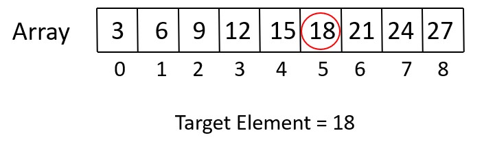
Sorted Array (Values) :- [3, 6, 9, 12, 15, 18, 21, 24, 27]
Target Element :- 18
Here’s the step-by-step dry run of the algorithm
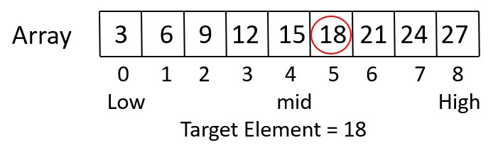
Begin with a sorted array: [3, 6, 9, 12, 15, 18, 21, 24, 27]
Initialize two variables ‘Low’ and ‘High’ and place them at the beginning and end of the array.
Low = index 0 (points to the first element, which is 3)
High = index 8 (points to the last element, which is 27)
Check if (High – Low > 1). In this case, it is true.
.
Iteration 1
Mid = Low + (High – Low) / 2 = 0 + (8 – 0)/ 2 = 4
.
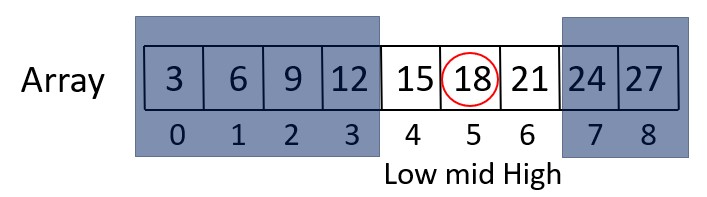
Check if values[mid] <= target element,
This is true because values[4] is 15, which is smaller than 18.
Update Low to be equal to mid (Low = mid = 4), so
Low = 4, and High = 8.
.
Iteration 2
Check if (High – Low == 1). In this case, it is true.
Calculate the midpoint:
Mid = Low + (High – Low) / 2 = 4 + (8 – 4)/ 2 = 6

.
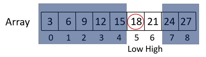
Check if values[mid] <= target element,
This is true because values[6] is 21, which is greater than 18.
Update High to be equal to mid (High = mid = 6), so
Low = 4, and High = 6.
.
Iteration 3
Check if (High – Low == 1) is true. In this case, it is true.
Calculate the midpoint:
Mid = Low + (High – Low) / 2 = 4 + (6 – 4)/ 2 = 5
.
Check if values[mid] <= target element,
This is true because values[5] is 18, which is equal to 18.
Update Low to be equal to mid (Low = mid = 5), so Low becomes 5, and High is 6.
.
Iteration 4
Check if (High – Low == 1) is true. In this case, it is false.
Stop searching.
.
By Checking Value[Low] == 18, we conclude that “Element found at location 5. Successful Search.”
.
Source Code for Ubiquitous Search
BOOKS