Types of Problems

Introduction

.

In computer science, computational complexity theory is used to classify problems based on how difficult they are to solve.

It helps us understand how much time and space (memory) an algorithm will take to solve a problem as the input size increases. Some problems are easy to solve, while others are very difficult and take a long time to find a solution.

We are interested in the hardness of the problem.

.

Types of Problems

(A) Some problems cannot be solved, no algorithm can be made for them, and they cannot even be formally defined. Such problems are infinite, abstract, or vague, for which there can be no clear rules or framework.

Example –

Q1 – “What is happiness?”
There is no definite answer to this question because each person’s definition of happiness is different. We cannot solve it using algorithms or mathematical rules, nor can we formally define it.
Q2 – “What is the best art?”
This question also cannot be clearly defined because the beauty or quality of art depends on the individual. There is no formula or algorithm to measure it.

.

(B) Some problems can be formally defined, but it is not possible to solve them through a computer or algorithm. These problems are called undecidable problems. No algorithm can provide a correct solution for all inputs in such cases.

Example –

Q1 – Automatic Computation by Programming

Creating a program that can solve all mathematical problems. This can be formally defined, but there is no algorithm that can provide correct answers for all possible mathematical questions.

Q2 – Tiling Problem  

This problem involves covering a surface with specific tiles without leaving any gaps. It can be defined formally, but in some cases, it is impossible to solve.

.

(C) Some problems can be theoretically solved, but they require such a large number of computational resources that solving them practically is not feasible. These problems are called intractable or infeasible

Example –

Q1 – Traveling Salesman Problem

In this problem, a salesman must visit several cities and find the shortest route. Although it can be solved theoretically, as the number of cities increases, the time and resources needed to calculate the solution grow so large that it becomes impractical.

Q2 – Open Halting Problem
This problem tries to identify whether a given program will run forever or stop eventually. While it can be theoretically defined, it is practically impossible to solve.

.

(D) These are problems that can be solved computationally and are not considered theoretically difficult. The key characteristic of these problems is that for each instance, a deterministic Turing machine exists that can solve the problem, with its time complexity being a polynomial function of the problem’s size.

Examples –

Q1 – Sorting algorithms (such as Merge Sort, Quick Sort), finding the shortest path in graphs (Dijkstra’s Algorithm), and searching (Binary Search).

.

(E) This class of problems is not known to have an efficient algorithm that runs in polynomial time (deterministic) or non-polynomial time (non-deterministic).

Example –

Q1 – Boolean satisfiability problem (SAT)

The SAT problem asks if there is an assignment of variables that satisfies a given Boolean formula.

SAT is in NP because, given a solution, you can verify it quickly (in polynomial time).

However, it is not known whether it can be solved in polynomial time by a deterministic algorithm, meaning it’s unclear if SAT belongs to P.

.

.

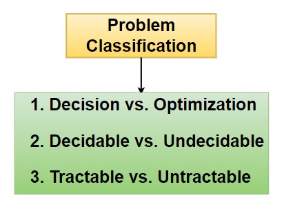
Problem Classification

When classifying problems in computer science, several classifications are commonly used, such as:

.

1. Decision Problems vs. Optimization Problems

Decision Problems – A decision problem asks a yes/no question about an instance of a problem. The goal is to determine whether a certain condition is met.

Example – “Is there a path from point A to point B in a graph?” The answer is either “yes” (a path exists) or “no” (no path exists).

1. Boolean Satisfiability Problem (SAT)
   Is there a way to assign truth values to variables so the formula is true? (Yes/No)
2. Vertex Cover
   Can we select a set of vertices of size ≤ k to cover all edges in the graph? (Yes/No)
3. Hamiltonian Cycle
   Does the graph contain a cycle visiting every vertex exactly once? (Yes/No)
4. Graph Coloring
   Can the graph be colored with k colors such that no two adjacent vertices share the same color? (Yes/No)
5. Subset Sum
   Is there a subset of numbers that sums to a target value? (Yes/No)
6. Knapsack (0/1 decision version)
   Can items be selected to exactly meet a given weight and value limit? (Yes/No)
7. Clique Problem
   Does the graph contain a complete subgraph (clique) of size k? (Yes/No)
8. Shortest Path (decision version)
   Is there a path between two vertices with a total distance ≤ d? (Yes/No)
9. Travelling Salesman Problem (decision version)
   Can the salesman visit all cities with a total distance ≤ d? (Yes/No)

Each problem asks if a specific condition is met, leading to a simple “yes” or “no” answer, making them decision problems.

.

Optimization Problems – An optimization problem seeks to find the best solution from all feasible solutions.

In an optimization problem, you aim to either –

• Maximize a certain value (e.g., profit, efficiency).
• Minimize a certain value (e.g., cost, distance, time).

under certain constraints.

Example – “What is the shortest path from point A to point B in a graph?” The answer is a specific path that has the minimum total distance or cost.

1. Dijkstra’s Algorithm
   Finds the shortest path in a graph, minimizing the total distance.
2. Bellman-Ford Algorithm
   Minimizes the shortest path even with negative weights.
3. Floyd-Warshall Algorithm
   Finds the shortest paths between all pairs of vertices, minimizing total distance.
4. Prim’s Algorithm
   Minimizes the total edge weight in a minimum spanning tree.
5. Kruskal’s Algorithm
   Minimizes the total edge cost in a minimum spanning tree.
6. Branch and Bound
   Optimizes solutions by pruning non-optimal paths to minimize/maximize outcomes.
7. Dynamic Programming (Knapsack Problem)
   Maximizes the value of items within a weight limit.
8. Christofides Algorithm
   Minimizes the total travel distance in the Traveling Salesman Problem.

Each problem focuses on achieving the best (optimized) solution, whether it’s minimizing distance, cost, or maximizing value.

.

2. Decidable vs. Undecidable Problems

Decidable Problems – A problem is decidable if there is an algorithm that can provide a yes/no answer for every input in a finite amount of time.

In other words, a decidable problem can always be solved by an algorithm that halts after a certain number of steps, regardless of the input size.

Decidable problems are also known as solvable problems because they can be completely solved using a deterministic method.

Example –

1. Checking if a number is prime
   The algorithm halts and gives a yes/no answer.
2. Determining if a string is accepted by a finite automaton
   The automaton halts and decides whether the string is accepted.
3. Linear Search Algorithm
   Halts after finding the target or confirming it is not in the array.
4. Binary Search Algorithm
   Provides a yes/no answer by halting once the target is found or determined absent.
5. Depth-First Search (DFS)
   Halts when it finds the target node or completes the traversal.
6. Breadth-First Search (BFS)
   Halts after exploring all nodes or finding the target.
7. Deterministic Finite Automaton (DFA)
   Determines acceptance of a string by halting after reading the input.
8. Merge Sort
   Sorts a list and halts after completion.
9. Quicksort
   Sorts an array and halts when sorting is done.
10. Bellman-Ford Algorithm
    Finds the shortest path and halts after determining if it is feasible.
11. Dijkstra’s Algorithm
    Halts after finding the shortest path between nodes.
12. Kruskal’s Algorithm
    Halts when it finds the minimum spanning tree of a graph.
13. Prim’s Algorithm
    Halts after constructing the minimum spanning tree.
14. Warshall’s Algorithm
    Halts when it finds the transitive closure of a graph.
15. Topological Sorting Algorithm
    Halts after sorting the nodes of a directed acyclic graph.
16. Huffman Coding Algorithm
    Halts when the optimal prefix code is generated.
17. Longest Common Subsequence (LCS) Algorithm
    Halts after finding the LCS between two sequences.

These problems can be fully solved using deterministic algorithms that ensure a result within a finite number of steps.

.

Undecidable Problems – A problem is undecidable if no algorithm can give a correct yes/no answer for all possible inputs. There is no general solution that works for every instance.

These problems are beyond the capability of any computational model to solve universally.

Example – The Halting Problem, which asks whether a program will halt (stop running) or run forever on a given input, is undecidable.

1. Halting Problem
   Determines whether a program will halt or run forever on a given input; no algorithm can solve this for all cases.
2. Tiling Problem
   Asks whether a given set of tiles can completely cover a plane without overlaps or gaps; no algorithm can decide this universally.
3. Post Correspondence Problem
   Involves finding a sequence of pairs that matches two strings; no algorithm guarantees a solution for all instances.
4. Rice’s Theorem
   States that any non-trivial property of the languages recognized by Turing machines is undecidable.
5. The Liar Paradox
   Involves statements that cannot be consistently classified as true or false; no algorithm can resolve all variations.
6. The Problem of the Greatest Common Divisor
   While the GCD itself can be found, deciding if two arbitrary numbers have a GCD that meets specific criteria can be undecidable.
7. The Problem of Finding a Regular Expression for a Language
   Determining a regular expression that defines a given language is undecidable in general cases.
8. The Problem of Satisfiability of First-Order Logic
   Deciding whether a first-order logic statement is satisfiable is undecidable in many cases.
9. The Problem of Infinite Loops in Algorithms
   No algorithm can determine whether every possible algorithm will enter an infinite loop or not.
10. The Problem of Non-terminating Programs
    Deciding if a program will terminate or continue running indefinitely cannot be universally solved.

These problems demonstrate the limitations of algorithms and computational models, highlighting the existence of questions that remain unsolvable.

3. Tractable vs. Intractable Problems

Tractable Problems – Tractable problems are problems that can be solved efficiently, meaning their solution can be found in polynomial time by an algorithm.

In other words, as the size of the input increases, the time required to solve the problem grows at a reasonable rate, such as n² or n³, where n is the size of the input.

These problems are considered feasible or practically solvable because their solution time remains manageable even for large inputs.

Examples –

1. Bubble Sort
   A simple sorting algorithm with a time complexity of O(n²).
2. Merge Sort
   A divide-and-conquer sorting algorithm with a time complexity of O(nlogn).
3. Quick Sort
   An efficient sorting algorithm with an average-case time complexity of O(nlog n).
4. Binary Search
   An algorithm for finding an element in a sorted array with a time complexity of O(log n).
5. Dijkstra’s Algorithm
   An algorithm for finding the shortest path in a graph with non-negative edge weights, operating in O(V²) or better.
6. Prim’s Algorithm
   A greedy algorithm for finding the minimum spanning tree in a graph, with a time complexity of O(Elog V).
7. Kruskal’s Algorithm
   Another greedy algorithm for finding the minimum spanning tree, with a time complexity of O(Elog E).
8. Dynamic Programming (e.g., Fibonacci Sequence)
   Algorithms that solve problems by breaking them down into simpler subproblems, such as computing Fibonacci numbers in O(n) time.
9. Breadth-First Search (BFS)
   An algorithm for traversing or searching tree or graph data structures, with a time complexity of O(V+E).
10. Depth-First Search (DFS)
    An algorithm for traversing or searching tree or graph data structures, with a time complexity of O(V+E).

Tractable problems are essential in computer science because they can be solved in a reasonable amount of time, making them applicable in real-world scenarios.

.

Intractable Problems – are problems that cannot be solved efficiently within a reasonable amount of time as their size grows. These problems typically require algorithms that run in non-polynomial time (e.g., exponential time or factorial time), making them impractical to solve for large inputs.

In other words, even though there might be an algorithm to solve the problem, the time required to compute the solution becomes so large that it is not feasible for real-world applications.

Examples –

1. Traveling Salesman Problem (TSP)
   Finding the shortest route visiting each city requires evaluating all possible routes, leading to factorial time complexity.
2. Knapsack Problem
   Determining the best combination of items to maximize value while staying within a weight limit can require checking exponential combinations.
3. Hamiltonian Cycle Problem
   Deciding if a cycle exists that visits every vertex exactly once involves exploring many potential paths, making it NP-complete.
4. Graph Coloring Problem
   Assigning colors to vertices so that no two adjacent vertices share the same color requires checking numerous color arrangements, resulting in NP-hard complexity.
5. Subset Sum Problem
   Finding a subset that sums to a specific target requires evaluating many possible subsets, leading to pseudo-polynomial time complexity.
6. Integer Linear Programming
   Solving linear equations with integer constraints is NP-hard, often requiring extensive computation for large inputs.
7. Job Scheduling Problem
   Optimizing job schedules can involve evaluating many possible sequences, which can grow exponentially with the number of jobs.
8. Clique Problem
   Finding a complete subgraph requires examining all possible combinations of vertices, leading to NP-completeness.
9. Set Cover Problem
   Identifying the smallest number of sets to cover a universal set requires evaluating various combinations, which is NP-hard.
10. Partition Problem
    Deciding if a set can be split into two equal-sum subsets involves checking multiple combinations, leading to NP-completeness.

These problems become impractical for large inputs due to their significant computational requirements, often necessitating the use of approximation or heuristic methods.

.

We understand that the time needed to solve a problem depends on its complexity. For easier problems, we can find algorithms that solve them in polynomial time, meaning the time grows at a manageable rate as the input size increases. However, for harder problems, the time required often grows exponentially, making them much more difficult to solve.

When we encounter problems that have no algorithmic solution, we cannot even define a time limit for solving them. In such cases, the problem is considered undecidable, and we can’t expect to find a solution in any reasonable amount of time.

In the upcoming post, we will explore the intricate landscape of computational complexity by discussing the concepts of P, NP, NP-Complete, and NP-Hard problems.

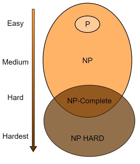
These classifications are fundamental to understanding how different problems can be approached in the realm of computer science.

The discussion will shed light on why certain problems are considered more challenging than others, the implications of these classifications for real-world applications, and the ongoing efforts in the field to find efficient solutions.