Traveling Salesman Problem

Distribute Education like Computer Geek

Introduction

.

The Traveling Salesman Problem (TSP) is a classic problem in computer science and mathematics. The goal is to find the shortest possible route that allows a salesman to visit each city exactly once and return to the starting city.

.

It’s a problem that can be solved using different methods, and one effective approach is the Branch and Bound algorithm.

The TSP can be solved using various methods

  1. Brute Force – Check all possible routes and choose the shortest one. This method guarantees the optimal solution but is impractical for large datasets due to its high computational cost.
  2. Greedy Algorithms – Heuristics that make local optimal choices at each step to find a global optimum. It is also called Nearest Neighbour Problem.
  3. Dynamic Programming – Optimizes the problem by solving subproblems and combining their solutions. It is also called Held-Karp algorithm.
  4. Branch & Bound Approach – breaking the problem into smaller subproblems (branching) and calculating a lower bound for each subproblem. If the lower bound exceeds the current best solution, that branch is pruned (ignored).
  5. Approximation Algorithms – Provides near-optimal solutions in a reasonable time, useful for large instances. It is also called Christofides Algorithm.

We first solve the Travelling Salesman Problem by Greedy algorithm, then solve by Dynamic Programming and now we are solving it by Branch & Bound algorithm.

.

Problem Statement

You are given a set of n cities and a distance matrix that represents the cost of traveling between each pair of cities. The goal is to find the shortest possible route that visits each city exactly once and returns to the starting city. This is known as the Traveling Salesman Problem (TSP).

Using the Branch and Bound approach, your task is to find the optimal solution (shortest route) for the TSP.

The algorithm should

  1. Explore all possible routes but efficiently eliminate paths that cannot lead to the optimal solution (using bounds).
  2. Return the shortest route along with the total cost of that route.

.

History

Branch and Bound was introduced as an exact method to solve TSP in the 1960s. The method was proposed by A. H. Land and A. G. Doig in 1960 to solve integer programming problems, but its powerful ability to reduce the search space made it applicable to other combinatorial problems, including TSP.

In 1980s-1990s, improved bounding techniques and computational power allow for larger TSP instances to be solved using Branch and Bound.

In 2000s-Present, Branch and Bound continues to be used alongside other algorithms, and new hybrid approaches are developed for solving modern variations of TSP, like mapping DNA sequence and protein folding.

.

TSPAlgorithm
  1. Initialize
  • Start from an initial node (let’s call it start).
  • Calculate the lower bound (LB) by summing the two smallest outgoing edge costs from the starting node, and divide this sum by 2.
  1. Create Branches
  • At the 0th level, create branches to each of the remaining unvisited nodes.
  • For each branch, calculate the lower bound (LB) by updating the cost and sum of outgoing edges from the new node.
  • Prune the branches where the lower bound exceeds the minimum lower bound so far.
  1. Explore Next Level
  • From the current node with the smallest lower bound, create new branches to the unvisited nodes.
  • For each new branch, recalculate the lower bound considering the added cost of visiting that node.
  • Continue to prune paths where the lower bound is higher than the smallest found so far.
  1. Repeat Branching
  • Keep expanding branches from the current node to the next unvisited nodes, recalculating the lower bounds at each step.
  • Prune all branches where the lower bound exceeds the minimum lower bound.
  1. Complete the Tour
  • Continue expanding until all nodes have been visited. Once the last node is visited, return to the start node to complete the cycle.
  • Calculate the total cost of the tour and compare it to the lowest lower bound found in previous branches.
  1. Solution
  • The final solution will be the path that visits all nodes exactly once and returns to the start node, with the minimum total cost.

Example

Travelling Salesman Problem

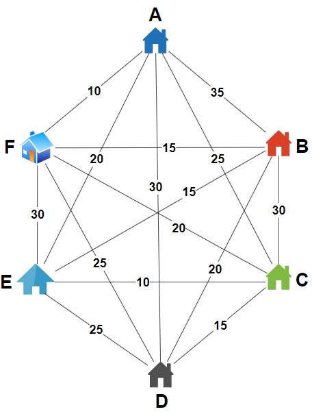
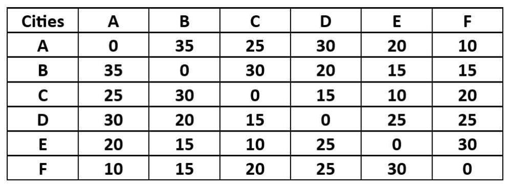
Example Distance Matrix
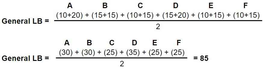
Travelling Salesman Problem adjacency matrix

Compute Lower bound

Lower bound = (Sum of two smallest distance edges) / 2

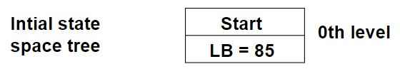
Step 1 – You have to compute General lower bound.

Travelling Salesman Problem branch & bound Lower Bound

.

So, its general lower bound is 85, means if you work upon any algorithm and by any method, the cost is not less than general lower bound. It will be equal to or greater than 85.

Travelling Salesman Problem branch & bound Graph 1

.

Step 2 – Compute Lower Bound from city A

Travelling Salesman Problem branch & bound lower bound from city A

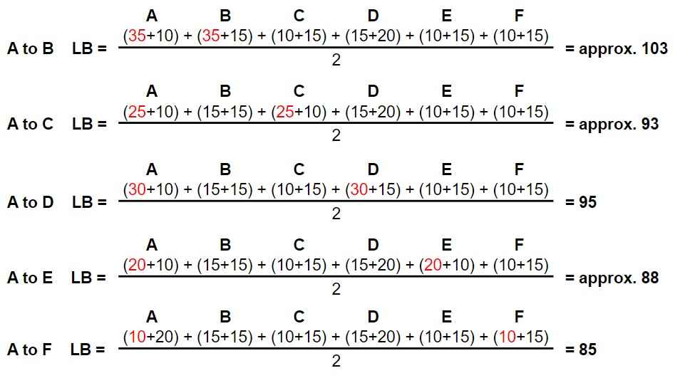
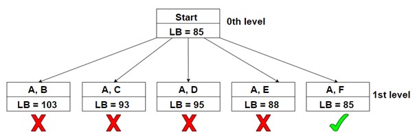
We have created paths from city A to all the other cities, and the lowest cost was from city A to city F. Therefore, we will travel from A to F because its lower bound is 85. The other cities have a higher lower bound, so we will not choose them. We have pruned those paths using the branch and bound method.

Travelling Salesman Problem branch & bound Graph 2

.

Step 3 – Compute Lower Bound from city F

From city A to city F, you have to use 10 costs, as given in the graph and is denoted with red colour. Also, the computation involved is in blue colour.

Travelling Salesman Problem branch & bound 3

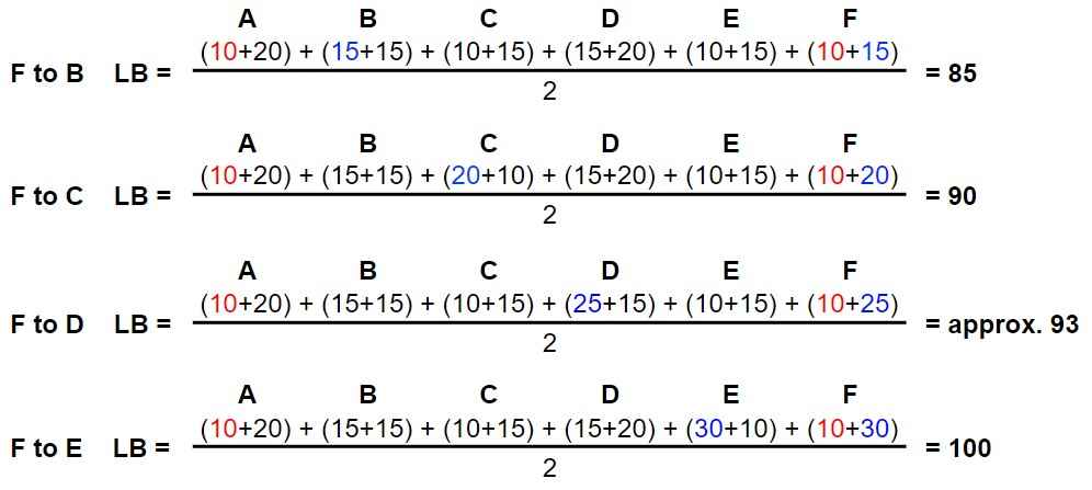
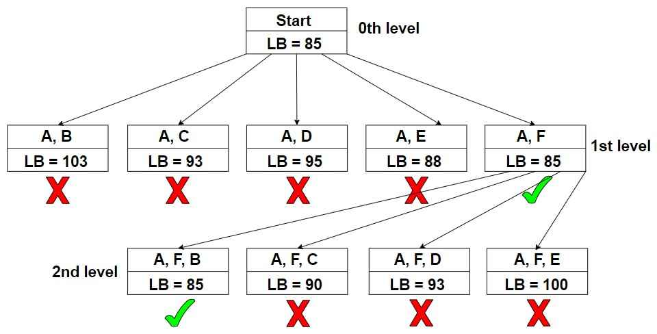
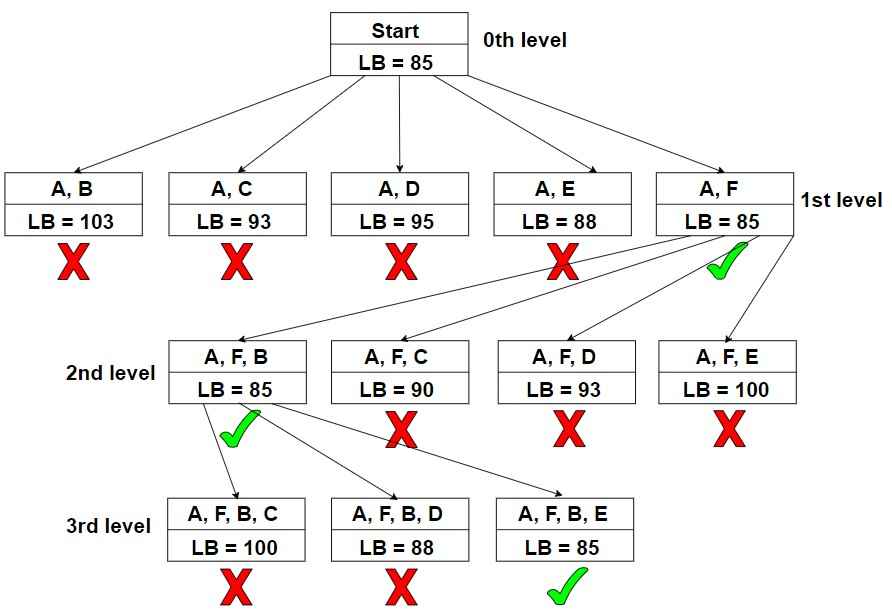
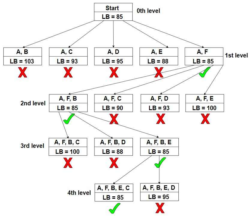
We have created paths from city F to all the other cities, and the lowest cost was from city F to city B. Therefore, we will travel from F to B because its lower bound is 85. The other cities have a higher lower bound, so we will not choose them. We have pruned those paths using the branch and bound method.

Travelling Salesman Problem branch & bound Graph 3 (2)

.

Step 4 – Compute Lower Bound from city B

From city A to city F and city F to city B, you have to use 10 + 15 = 25 cost, as given in the graph and is denoted with red colour. Also, the computation involved is in blue colour.

Travelling Salesman Problem branch & bound 4 (2)

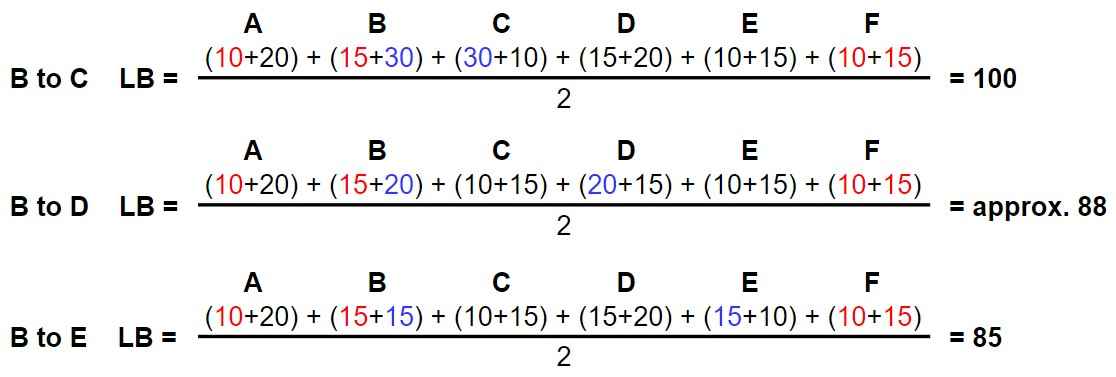
We have created paths from city B to all the other cities, and the lowest cost was from city B to city E. Therefore, we will travel from B to E because its lower bound is 85. The other cities have a higher lower bound, so we will not choose them. We have pruned those paths using the branch and bound method.

Travelling Salesman Problem branch & bound Graph 4 (2)

.

Step 5 – Compute Lower Bound from city E

From city A to city F, city F to city B, and city B to city E, you have to use 25 + 15 = 40 cost, as given in the graph and is denoted with red colour. Also, the computation involved is in blue colour.

Travelling Salesman Problem branch & bound 5 (2)

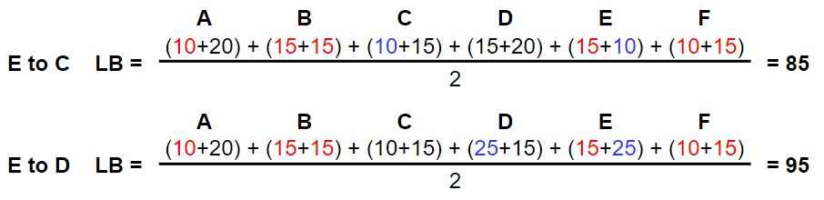
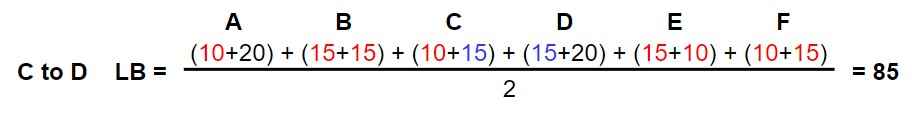
We have created paths from city E to all the other cities, and the lowest cost was from city E to city C. Therefore, we will travel from E to C because its lower bound is 85. The other cities have a higher lower bound, so we will not choose them. We have pruned those paths using the branch and bound method.

Travelling Salesman Problem branch & bound Graph 5 (2)

.

Step 6 There is only one city left, that is, city D. The cost require from city C to city D is 15. There is only one lower bound, so no pruning is there.

Travelling Salesman Problem branch & bound 6 (2)

Also, from city D to city A, the lower bound or cost is 30.

Travelling Salesman Problem branch & bound 7 (2)

Travelling Salesman Problem branch & bound

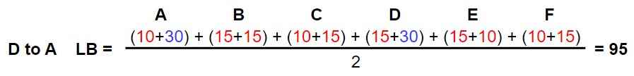
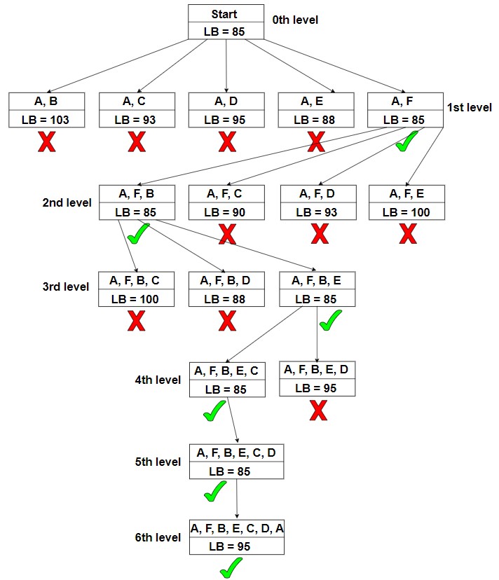
Therefore, path is A -> F -> B -> E -> C -> D -> A, and the lower bound or the total cost is 95.

.

Source Code for TSP using Branch & Bound
Time Complexity

Worst-Case Time Complexity – The time complexity of the Branch and Bound algorithm for TSP is generally exponential. In the worst case, it can be O(n!), where n is the number of cities. This is because the algorithm explores a large number of possible routes to find the optimal solution.

Average-Case Time Complexity – The average-case time complexity can be better than the worst-case but is still exponential. It depends on the specific problem instance and the efficiency of the branching strategy and bounding function used.

.

Space Complexity

The space complexity of the Branch and Bound algorithm is also exponential, O(n!), due to the need to store information about all potential routes and the corresponding bounds. The actual space required can be somewhat less if the algorithm employs pruning strategies that reduce the number of routes stored.

.

Applications
  • Logistics and Route Optimization – Used for optimizing delivery routes in logistics and supply chain management to minimize travel costs and time.
  • Manufacturing – Helps in scheduling tasks on machines to minimize the total completion time.
  • Telecommunications – Applied to network design and optimization to ensure efficient communication and minimize costs.
  • Travel Planning – Assists in planning travel itineraries to visit multiple destinations in the shortest possible time.
  • Robotics – Used in path planning for robots that need to visit multiple points or locations efficiently.

Test Yourself

Q1- What is the lower bound in the Branch and Bound algorithm for TSP?

In the Branch and Bound algorithm for the Traveling Salesman Problem (TSP), the lower bound is an estimate of the minimum possible cost to complete the tour from a given node (partial solution). It helps to decide whether to prune (cut off) certain branches of the solution tree.

The lower bound is calculated by:

  1. Selecting the two smallest outgoing edges (or costs) from each city that has not yet been visited in the partial tour.
  2. Summing up these minimum edges for all cities gives the lower bound estimate.

This lower bound represents the best possible outcome from that node onward and is used to avoid exploring branches where the cost exceeds the current best-known solution. If a branch’s lower bound is greater than the best-known tour cost, that branch is pruned.

Q2- Why do we prune branches in the Branch and Bound algorithm?

We prune branches in the Branch and Bound algorithm to reduce the search space and improve efficiency. The primary reasons for pruning are:

  1. Avoid Exploring Inefficient Paths – If a branch’s lower bound (minimum possible cost) is higher than the cost of the current best-known solution, it means that this branch cannot lead to a better solution. Pruning avoids unnecessary exploration of such paths.
  2. Save Time and Resources – By cutting off branches that are unlikely to lead to optimal solutions, the algorithm reduces the number of nodes it needs to evaluate, saving time and computational resources.
  3. Focus on Promising Solutions – Pruning helps the algorithm focus on more promising branches that have the potential to lead to the best or optimal solution, speeding up the search process.
Q3- How does Branch and Bound differ from the Greedy algorithm for TSP?

Branch and Bound and the Greedy algorithm differ significantly in their approach to solving the Traveling Salesman Problem (TSP).

The Greedy algorithm follows a straightforward method by making the locally optimal choice at each step, aiming to find a short-term solution that seems best at that moment. It does not reconsider previous decisions and often fails to find the global optimal solution for TSP.

On the other hand, Branch and Bound systematically explores different solutions by dividing the problem into smaller subproblems (branches). It calculates a lower bound for each branch, helping to eliminate or “prune” branches that cannot lead to a better solution. This ensures that all possible routes are considered, but only the most promising ones are explored in depth, leading to an optimal solution.

While the Greedy algorithm is faster but less accurate, Branch and Bound is slower but guarantees finding the best possible solution.

Q4- Can Branch and Bound guarantee the optimal solution for TSP?

Yes, Branch and Bound can guarantee the optimal solution for the Traveling Salesman Problem (TSP).

This method systematically explores all possible solutions by breaking down the problem into smaller subproblems and calculating bounds to prune branches that cannot lead to a better solution. By using techniques such as bounding functions and pruning, Branch and Bound ensures that every potential route is considered, but only the most promising branches are pursued.

This comprehensive exploration, combined with the elimination of suboptimal branches, allows Branch and Bound to find the true optimal solution, provided it has enough time and computational resources to explore all necessary branches.

Q5- What is the significance of finding two smallest edges in the lower bound calculation?

Finding the two smallest edges from each node provides an estimate of the cost to visit all cities, which helps in setting a lower bound for the current subproblem.

Q6- In what cases might the Branch and Bound algorithm be less efficient for solving TSP?

Branch and Bound can be less efficient when the problem size grows significantly, as it still explores many branches even with pruning. For very large datasets, it may become impractical.

Q7- Why is the initial bound important in Branch and Bound for TSP?

The initial bound sets a reference for pruning future branches. A tighter initial bound can lead to more efficient pruning and a faster solution.

Q8- What happens if we choose a poor initial bound in Branch and Bound?

A poor initial bound may lead to less efficient pruning, which increases the search space and computation time.

like we did in the example. we know that from city A, the minimum cost would be 95. But this is only for city A and this is the optimum answer. 

The Held-Karp algorithm having the same graph calculates that the graph will be travelled in cost 90. B -> F -> A -> E -> C -> D -> B

Q9- Can Branch and Bound handle asymmetric TSP (where the cost from city A to city B differs from B to A)?

Yes, the Branch and Bound method can handle both symmetric and asymmetric TSP by adjusting the cost matrix accordingly.

Q10- What is the main purpose of the Branch and Bound method?
  1. To explore all possible solutions without pruning.
  2. To greedily select the nearest neighbor.
  3. To explore all solutions and prune branches that cannot lead to the optimal solution.
  4. To randomly select routes.

Ans – (3)

Explanation – Branch and Bound explores all solutions but uses pruning to discard paths that exceed the current best solution.

Q11- Why does the Branch and Bound algorithm use pruning?
  1. To find local optimums.
  2. To explore all possible branches without missing any.
  3. To avoid paths that exceed the current best solution.
  4. To randomly skip paths.

Ans – (3)

Explanation – Pruning helps to avoid paths where the lower bound exceeds the best-known solution, making the algorithm more efficient.

Q12- In the context of TSP, what is a branch?
  1. A part of a tree that represents multiple solutions.
  2. A partial solution that represents a specific path choice from the current node.
  3. A way to eliminate solutions.
  4. A recursive function call.

Ans – (2)

Explanation – A branch represents a partial solution or choice of path from the current node to the next possible cities.

BOOKS

Algorithm T H CoremanAlgorithm by Udit AgarwalAlgorithm Ellis HorowitzData Structure & Algorithm Made Easy Narasimha

Â