Quick Sort

Distribute Education like Computer Geek

Introduction

.

Quick Sort is one of the most widely used sorting algorithms, based on the Divide and Conquer principle.

  1. It was invented by Tony Hoare in 1960.
  2. This algorithm is remarkable for its great efficiency and simplicity.
  3. The problem is broken down into smaller sub-problems, each one sorted individually, and then merged to form the final sorted list.
  4. Quick Sort often surpasses other sorting algorithms, such as Bubble Sort or Selection Sort, in most cases.
  5. In fact, quick sort is the fastest sorting algorithm in average case, its average case time complexity comes out as O(nlogn) but, in the worst case, quick sort time complexity comes out to be O(n2).
  6. Merge Sort is the fastest in the worst-case as its time complexity is O(nlogn).

.

History of Quick Sort Algorithm

Quick Sort, which is one of the most efficient and widely used sorting algorithms, has a very interesting history.

  1. It was invented in 1960 by Tony Hoare, a British computer scientist, while he was working on machine translation at Moscow State University.
  2. In his work on a Russian to English translation project, Tony Hoare encountered the problem of how to sort data efficiently.
  3. Applying the Divide and Conquer strategy to sorting problems, he found himself inventing the strategy of selecting a “pivot” element and partitioning the data around it. He invented Quick Sort.

Quick Sort was implemented on early computers, and because of its simplicity and speed, it was revolutionary. Now it has become a standard algorithm in computer science and is taught in most courses of algorithms and implemented in the system libraries of C++ STL, Python, and Java.

While Tony Hoare’s partitioning algorithm is efficient, it is also more complex to implement correctly. 

In Tony Hoare’s original partitioning algorithm

  1. Choose a pivot element (often the first or middle element). If the pivot is the last element, then it may cause Quicksort to go into an infinite recursion.
  2. Use two pointers, one starting at the left and the other at the right.
  3. Move the left pointer until an element larger than the pivot is found.
  4. Move the right pointer until an element smaller than the pivot is found.
  5. Swap these two elements and continue until the pointers meet

To simplify the implementation, we use the Nico Lomuto Partition Scheme. 

.

.

Working of Quick Sort
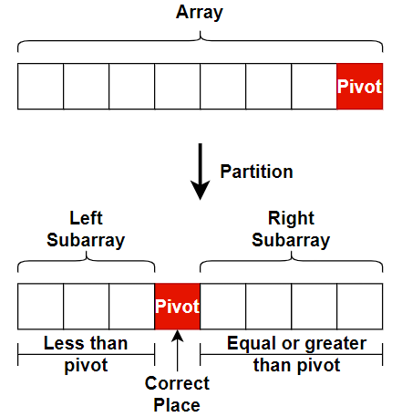
  1. Divide – Quick Sort works on the principle of choosing an element as a pivot and splits the array into two sub-arrays.

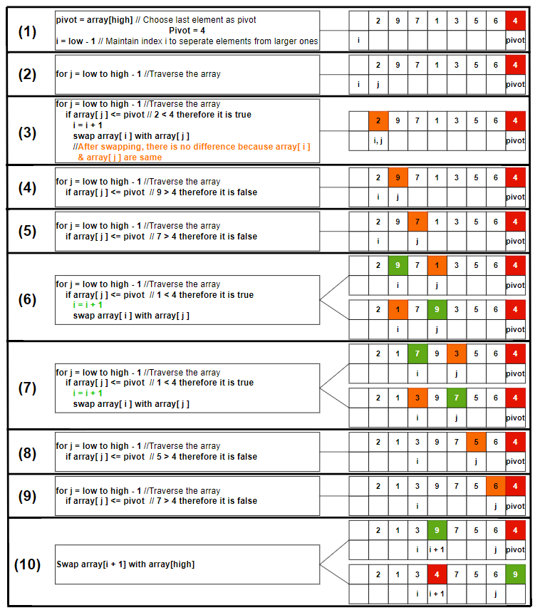
Partitioning Using Nico Lomuto Scheme Algorithm

function partition(array, low, high)

    pi = array[high] // Choose last element as pivot (pi)

    i = low – 1 // Maintain index i to separate elements from larger ones.

    for j = low to high – 1 // Traverse the array

        if array[j] <= pivot

            i = i + 1

            swap array[i] with array[j]

           // Swap smaller elements before the pivot

    swap array[i + 1] with array[high]

    return i + 1

By executing this partition scheme, the pivot is in correct position.

Quick Sort diagram

  1. Conquer – Recursively apply the same process to the left and right subarrays.

function quickSort(array, low, high)

    if low < high

        pi = partition(array, low, high)

        quickSort(array, low, pi – 1)

        quickSort(array, pi + 1, high)

  1. Combine – Since quick sort sorts in-place, there is no explicit combination step. The array becomes sorted as the recursion unwinds.

.

Example

Some professor says that the example given in Thomas H. Coreman is very complex and some says that quick sort algorithm given in this book is wrong because they are not able to solve the example given in this book.

So, we are taking same example but with some uniqueness.

Let take the array = {2, 9, 7, 1, 3, 5, 6, 4}

We use Nico Lomuto partition algorithm. Here is the step-by-step process.

.

Quick Sort

.

Here the partition is done and the pivot = 4 is in the correct position. All the numbers on the left of 4 are smaller than or equal to 4, and all the numbers on the right of 4 are greater than 4.

Small or equal numbers ≤ pivot = 4 < Greater numbers

The left subarray and the right subarray are not sorted, so we will first apply the Quick Sort algorithm to the left subarray.

.

Left Subarray = {2, 1, 3}

Quick Sort Left Subarray

.

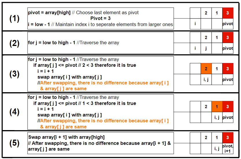
Pivot = 3 does not move after applying algorithm, it means that it is the greatest number in the array. We will apply the algorithm of quick sort to the left-left subarray.

.

Left-Left subarray = {2, 1}
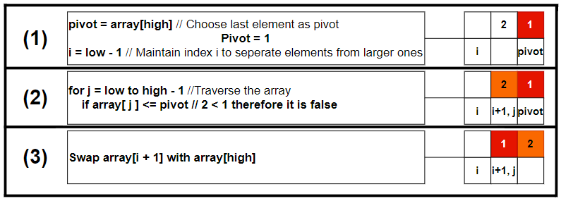
Quick Sort left-left subarray

.

Left subarray has no element, now we will apply algorithm on right subarray.

.

Right Subarray = {7, 5, 6, 9}
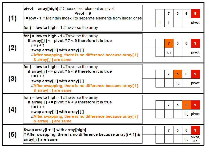
Quick Sort Right Subarray

.

Pivot = 9 does not move after applying algorithm, it means that it is the greatest number in the array. We will apply algorithm of quick sort to the right-left subarray.

.

Right-Left subarray = {7, 5, 6}
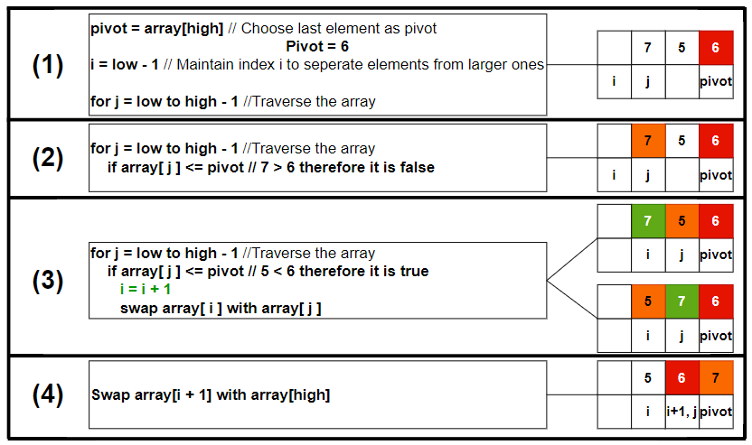
Quick Sort Right-Left Subarray

.

Here the partition is done and the pivot = 6 is in correct position. All the numbers in the left are smaller than or equal to 6, and all the numbers on the right is greater than 6, and there is only one number in left array and right array, so it is already sorted.

Combine – {1, 2}, {3}, {4}, {5, 6, 7}, {9}

The array is – {1, 2, 3, 4, 5, 6, 7, 9}

.

Source Code of Quick Sort

Time Complexity of Quick Sort

There are three cases best, average and worst, in which time complexity differs.

  • Best Case – When pivot divides the whole array into two equal partitions. Left subarray and right subarray have approximately n/2 elements.

T(n) = 2T(n/2) + O(n)


Solve this by master’s method.

It will give T(n) = O(nlogn)

So, when pivot is chosen so that it divides the whole array into two subequal parts then the time complexity is O(nlogn).


  • Average Case – The pivot divides the array into two subarrays, but not perfectly equal like the best case. One subarray has n/4​ elements, and the other has 3n/4.

This is because the pivot is selected randomly, and because of several recursive calls, the imbalance cancels out.

T(n) = T(k) + T(n−k−1) + O(n)


where, k is the number of elements in the left subarray. (n – k − 1) is the number of elements in the right subarray. O(n) is the time spent in partitioning.

This k is roughly the same as n/2. So, T(n) ≈ 2T(n/2) + O(n) will result in O(nlogn).


  • Worst CaseThe pivot is always the smallest or largest element, resulting in highly unbalanced partitions. One subarray contains n-1 elements and other subarray contains 0 (zero) elements.

T(n) = T(n-1) + O(n)

This will result in time complexity of O(n2).

.

Space Complexity

In the best case (balanced partitions) and average case, the recursion depth is O(log n), so the auxiliary space is O(log n).

In the worst case (highly unbalanced partitions), the recursion depth is O(n), so the auxiliary space is O(n).

.

Advantage
  1. Quick Sort is faster on average than other sorting algorithms like Bubble Sort or Insertion Sort.
  2. Quick Sort is an in-place sorting algorithm, meaning it does not require additional storage for sorting.
Disadvantage
  1. The worst-case time complexity is O(n2), which occurs when the pivot selection consistently results in unbalanced partitions.
  2. Quick Sort is not a stable sorting algorithm, meaning equal elements may not retain their relative order.
  3. Choosing the pivot poorly can significantly degrade performance.
  4. For very small datasets, the recursive overhead may make Quick Sort slower compared to simpler algorithms like Insertion Sort.

Test Yourself

Q1- Why is Quick Sort not considered a stable sorting algorithm?

Quick Sort is not considered a stable sorting algorithm because it does not preserve the relative order of equal elements in the input array. In other words, if two elements are equal, their relative order might change after the sorting process.

Before Sorting – [4a, 2, 4b, 3]

After Sorting – [3, 2, 4b, 4a]

Q2- Explain why the choice of pivot affects the performance of Quick Sort.
  • The choice of the pivot determines the balance of the partitions.
  • A well-chosen pivot results in partitions of approximately equal size, leading to a time complexity of O(nlogn).
  • Poor pivot choices, such as selecting the smallest or largest element, result in highly unbalanced partitions, increasing the number of recursive calls and degrading performance to O(n2).
  • Methods like random pivot selection or the median-of-three approach help mitigate this problem.
Q3- Why is Quick Sort preferred over Merge Sort for arrays but not for linked lists?
  • Quick Sort works well with arrays because it sorts in-place, minimizing space usage.
  • For linked lists, Quick Sort requires random access for efficient partitioning, which linked lists lack. Merge Sort, which relies on sequential access, is better suited for linked lists.
Q4- What are the advantages of Quick Sort over Merge Sort?

Quick Sort is in-place, requiring no additional memory, and has better performance for most real-world datasets due to reduced overhead.

Q5- Under what scenarios should Quick Sort be avoided?

Quick Sort should be avoided for datasets with high redundancy or when stability is required, as it may result in poor performance or incorrect relative ordering.

Q6- Who invented Quick Sort?
  1. Donald Knuth
  2. Tony Hoare
  3. Alan Turing
  4. Nico Lomuto

Ans – (2)

Explanation – Tony Hoare invented Quick Sort in 1960 while working on a translation project.

Q7- Which principle does Quick Sort use?
  1. Divide and Conquer
  2. Dynamic Programming
  3. Greedy Algorithm
  4. Backtracking

Ans – (1)

Explanation – Quick Sort breaks the array into subarrays around a pivot and recursively sorts them.

Q8- Which partition scheme is more efficient in practice?
  1. Hoare
  2. Lomuto
  3. Merge
  4. Radix

Ans – (1)

Explanation – Hoare’s scheme minimizes swaps and is generally faster than Lomuto’s scheme.

Q9- What happens in Quick Sort’s worst case?
  1. Balanced partitions
  2. Unbalanced partitions
  3. No recursion
  4. Extra memory is used

Ans – (2)

Explanation – Worst case occurs when the pivot is smallest or largest, leading to one-sided recursion.

Q10- Which case of Quick Sort has the highest recursion depth?
  1. Best case
  2. Average case
  3. Worst case
  4. None of the above

Ans – (3)

Explanation – Worst case leads to O(n) recursion depth.

Q11- In which scenario does Quick Sort perform the worst
  1. When the array is completely sorted
  2. When the array is reverse sorted
  3. When all elements are equal
  4. All of the above

Ans – (4)

Explanation – These scenarios lead to unbalanced partitions, causing O(n2) complexity.

BOOKS

Algorithm T H CoremanAlgorithm by Udit AgarwalAlgorithm Ellis HorowitzData Structure & Algorithm Made Easy Narasimha

Â