

Understanding Prim’s Algorithm
The algorithm was developed by Czech mathematician Vojtín Czernik in 1930 and later by computer scientists Robert C. Prim in 1957 and Edgard W. Dijkstra in 1959. Therefore, it is sometimes also called the Járnik algorithm, prim-Járnik algorithm, prime. -Dijkstra algorithm or DJP algorithm.
.
What is Prim’s Minimum Spanning Tree Algorithm?
Prim’s Algorithm is a greedy algorithm used for finding the minimum spanning tree (MST) of a connected, undirected graph.
- The goal of Prim’s algorithm is to connect all the vertices of the graph while minimizing the total weight of the edges in the spanning tree.
- The algorithm starts with an arbitrary vertex and grows the spanning tree by adding the shortest edge that connects a vertex in the tree to a vertex outside the tree at each step.
- The process continues until all vertices are included in the minimum spanning tree.
- Prim’s algorithm ensures that the resulting tree is acyclic and spans all the vertices with the least possible total edge weight.
.
Algorithm
- Begin with an arbitrary node.
- Find the shortest edge connecting any unvisited node to the current tree.
- Add the selected edge and the connected node to the tree.
- Repeat steps 2-3 until all nodes are included in the tree.
.
Working of Prim’s Algorithm
Imagine you have a network of houses, and you want to build roads between them with the least total distance.
Prim’s algorithm starts with a single node and adds the shortest edge that connects a new node to the existing structure at each step. It continues this process until all nodes are connected.

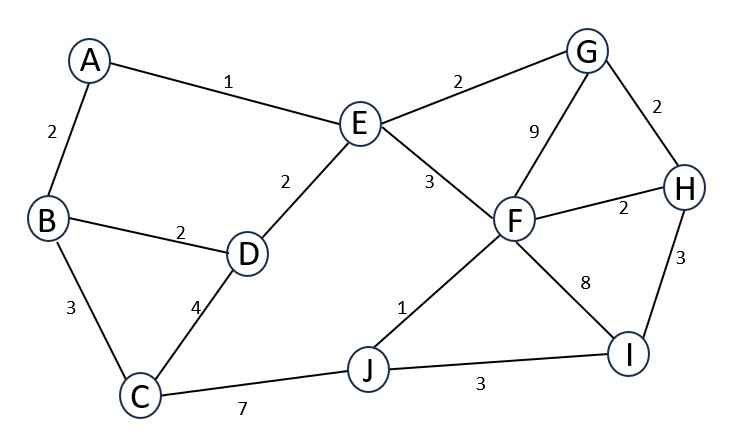
Let’s solve for the minimum spanning tree using Prim’s algorithm with the given graph –
Vertices: A, B, C, D, E, F, G, H, I, J
Edges with weights – 16
.
Initialization
Start with an arbitrary vertex, let’s say A.
Initialize an empty set T (the minimum spanning tree) and a priority queue or min-heap to store edges.
.
Adding Edges
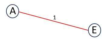
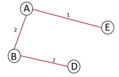
Add the minimum-weight edge connected to A, which is AE (weight = 1). Update T.
Now, add the next minimum-weight edge connected to A or E. So, the edges are {AB = 2, ED = 2, EG = 2, EF = 3}.
You have to select an edge of minimum weight which has one unvisited vertex, no cycles or loops in tree.
So, we select AB. Update T.

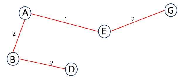
Now, add the next minimum-weight edge connected to A, B or E. So, the edges are {BD = 2, BC = 3, ED = 2, EG = 2, EF = 3}.
You have to select an edge of minimum weight which has one unvisited vertex, no cycles or loops in tree.
So, we select BD. Update T.
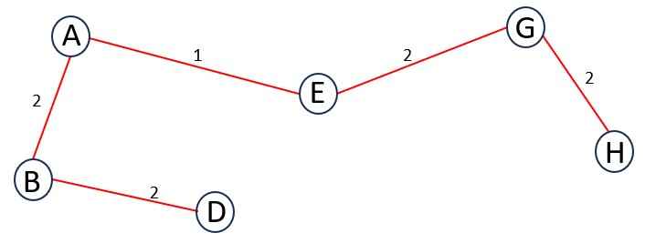
Now, add the next minimum-weight edge connected to A, B, D or E. So, the edges are {BC = 3, DC = 4, EG = 2, EF = 3}.
ED is not in the list because a cycle is formed.
You have to select an edge of minimum weight which has one unvisited vertex, no cycles or loops in tree.
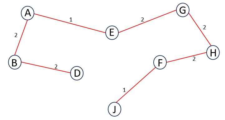
So, we select EG. Update T.
Now, add the next minimum-weight edge connected to A, B, D, E or G. So, the edges are {BC = 3, DC = 4, EF = 3, GF = 9, GH = 2}.
You have to select an edge of minimum weight which has one unvisited vertex, no cycles or loops in tree.
So, we select GH. Update T.
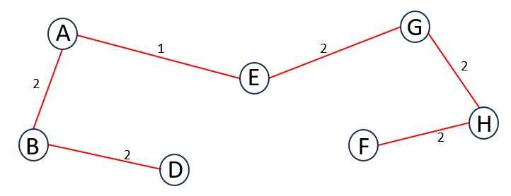
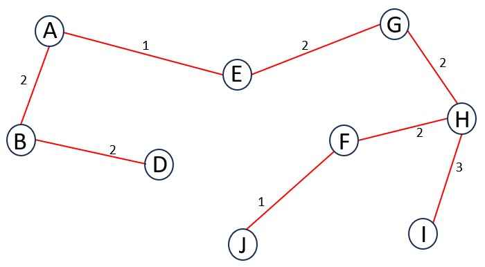
Now, add the next minimum-weight edge connected to A, B, D, E, G or H. So, the edges are {BC = 3, DC = 4, EF = 3, GF = 9, HF = 2, HI = 3}.
You have to select an edge of minimum weight which has one unvisited vertex, no cycles or loops in tree.
So, we select HF. Update T.
Now, add the next minimum-weight edge connected to A, B, D, E, G, H or F. So, the edges are {BC = 3, DC = 4, HI = 3, FJ = 1}.
EF and GF are not in the list because a cycle is formed.
You have to select an edge of minimum weight which has one unvisited vertex, no cycles or loops in tree.
So, we select FJ. Update T.
Now, add the next minimum-weight edge connected to A, B, D, E, G, H, F or J. So, the edges are {BC = 3, DC = 4, CJ = 7, HI = 3, FI = 8, JI = 3}.
You have to select an edge of minimum weight which has one unvisited vertex, no cycles or loops in tree.
So, we select HI. Update T.
Now, add the next minimum-weight edge connected to A, B, D, E, G, H, F, J or I. So, the edges are {BC = 3, DC = 4, CJ = 7}.
FI and JI are not in the list because a cycle is formed and there is no unvisited vertex.
You have to select an edge of minimum weight which has one unvisited vertex, no cycles or loops in tree.
So, we select BC. Update T.

The final minimum spanning tree.
The total weight of the minimum spanning tree is the sum of the weights of its edges.
Total Weight – 18
We can make multiple minimum spanning trees of prim’s with this graph and the total weight of their edges would be just 18 not more than that.
.
Source Code for Prim’s Algorithm
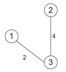
Q8- How to Find Minimum Spanning Tree Using Prim’s Algorithm?
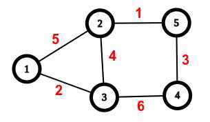
Let’s say vertex 1 is our starting point. You can choose any starting point.
Move 1
Visited Vertex(1) = Edges(5, 2)
We must select minimum weight, So, we choose 2.
The minimum spanning tree is
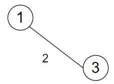
Total weight is 2.
Move 2
Visited Vertex(1, 3) = Edges(5, 4, 6)
We must select minimum weight, So, we choose 4.
The minimum spanning tree is
Total weight is 6.
Move 3
Visited Vertex(1, 3, 2) = Edges(1, 6)
We must select minimum weight, So, we choose 1.
The minimum spanning tree is

Total weight is 7.
Move 4
Visited Vertex(1, 3, 2, 5) = Edges(6, 3)
We must select minimum weight, So, we choose 3.
The minimum spanning tree is
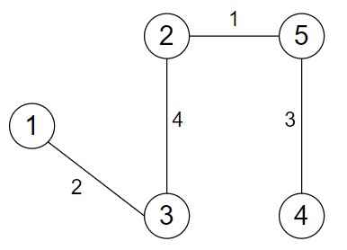
Total weight is 10.
Q9- Using Prim’s algorithm to construct a minimum spanning tree starting with node a, which one of the following sequences of edges represents a possible order in which the edge would be added to construct the minimum spanning tree?
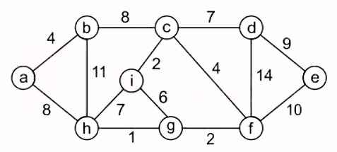
1. (a,b), (b,h), (g,h), (f, g), (c, f), (c, i), (c, d), (d, e)
2. (a,b), (b,c), (c,i), (c, f), (f, g), (g, h), (c, d), (d, e)
3. (a,b), (b,h), (g,h), (g, i), (c, f), (c, i), (c, d), (d, e)
4. (a,b), (g,h), (g,f), (c, f), (c, i), (f, e), (b, c), (d, e)
Ans – (2)
Explanation –

BOOKS