

Introduction
.
The Nearest Neighbour Problem (NNP) or Traveling Salesman Problem (TSP) by greedy method is a classic algorithmic problem in computer science and operations research.
The goal is simple – “Given a list of cities and the distances between them, find the shortest possible route that visits each city exactly once and returns to the starting point.”
This problem is crucial in fields like logistics, transportation, and manufacturing.
The TSP can be solved using various methods
- Brute Force – Check all possible routes and choose the shortest one. This method guarantees the optimal solution but is impractical for large datasets due to its high computational cost.
- Greedy Algorithms – Heuristics that make local optimal choices at each step to find a global optimum. It is also called Nearest Neighbour Problem.
- Dynamic Programming – Optimizes the problem by solving subproblems and combining their solutions. It is also called Held-Karp algorithm.
- Branch & Bound Approach – breaking the problem into smaller subproblems (branching) and calculating a lower bound for each subproblem. If the lower bound exceeds the current best solution, that branch is pruned (ignored).
- Approximation Algorithms – Provides near-optimal solutions in a reasonable time, useful for large instances. It is also called Christofides Algorithm.
We first solve the Travelling Salesman Problem by Greedy algorithm, that is Nearest Neighbour Problem.
.
Nearest Neighbour Problem Statement
“Given a set of n cities and the distances between every pair of cities, find a tour that visits each city exactly once and returns to the starting city.
The objective is to construct this tour using the Nearest Neighbour Algorithm, aiming to minimize the total distance travelled, though it may not yield the optimal solution.”
.
History
The concept of finding the nearest neighbour likely originates from the study of Voronoi diagrams in the 19th century by mathematicians like Georgy Voronoy. However, the computational aspects of the problem became a focus in the mid-20th century.
During this time, researchers began exploring the problem in the context of geographic information systems (GIS), clustering, and optimization.
In the 1970s, the problem became more formalized with the advent of computational geometry. The introduction of the k-d tree by Jon Bentley in 1975 was a significant breakthrough. The k-d tree is a data structure that allows efficient search for the nearest neighbour in a multidimensional space. During this period, the problem was also studied in operations research, particularly in the context of the Traveling Salesman Problem (TSP). The nearest neighbour heuristic became a popular method for generating approximate solutions to the TSP.
The nearest neighbour search problem also became crucial in machine learning, pattern recognition, and computer vision. For example, in k-nearest neighbours (k-NN) classification, the goal is to classify a data point based on the majority class of its nearest neighbours.
.
Algorithm NearestNeighborTSP(C, D)
Input –
C = {C1, C2, …, Cn} // Set of n cities
D = Distance matrix where D[i][j] is the distance between city Ci and city Cj
1. Let currentCity = C1 // Start from the first city
2. Mark currentCity as visited
3. Initialize tour = [currentCity]
4. Initialize totalDistance = 0
5. While there are unvisited cities
- Find the nearest unvisited city (Minimum Distance)
- Add the distance D[currentCity][nearestCity] to totalDistance
- Move to nearestCity
- Mark nearestCity as visited
- Append nearestCity to tour
- Set currentCity = nearestCity
6. Add the distance D[currentCity][C1] to totalDistance // Return to the starting city
7. Append the starting city C1 to the end of the tour
8. Output tour and totalDistance
.
Example –
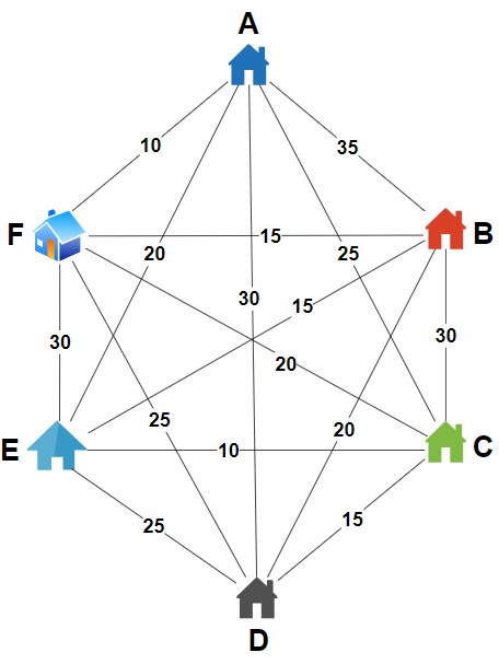
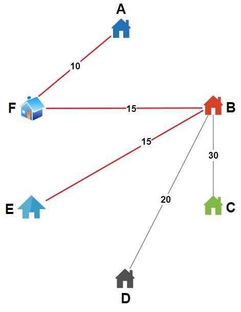
Example Distance Matrix
.
Find a tour that visits each city exactly once and returns to the starting city by always moving to the nearest unvisited city.
Steps
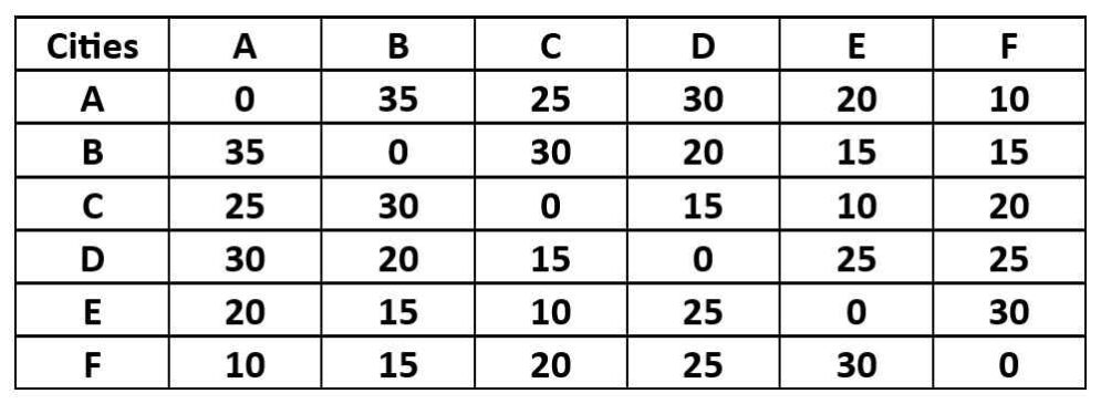
1. Initialization
- Start at City A.
- Mark City A as visited.
- Initialize tour with City A.
2. Iterative Process
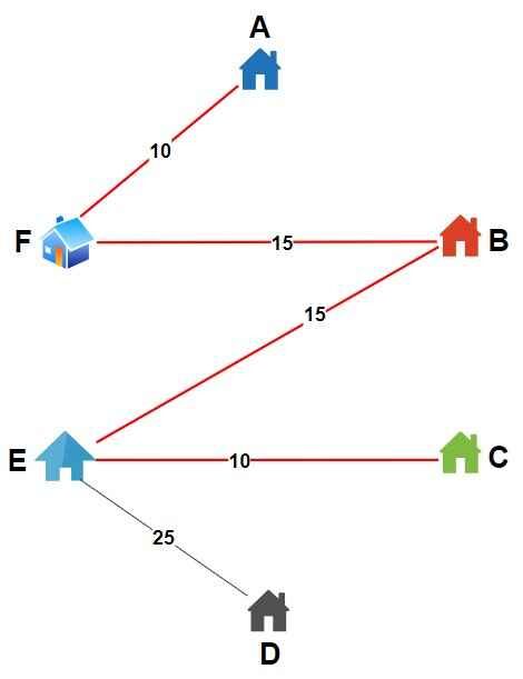
- From City A –
- Unvisited cities = B, C, D, E, F
- Distances is A → B = 35, A → C = 25, A → D = 30, A → E = 20, A → F = 10
- Nearest city, F (distance = 10)
- Move to F, mark F as visited.
- Total tour distance = 10
- From City A –
.
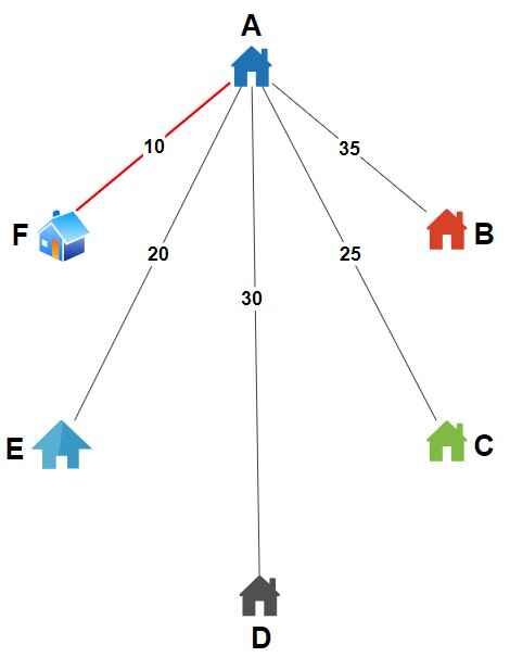
- From City F –
- Unvisited cities = B, C, D, E
- Distances is F → B = 15, F → C = 20, F → D = 25, F → E = 30
- Nearest city, B (distance = 15)
- Move to B, mark B as visited.
- Total tour distance = 10 + 15 = 25
.
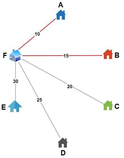
- From City B –
- Unvisited cities = C, D, E
- Distances is B → C = 30, B → D = 20, B → E = 15
- Nearest city, E (distance = 15)
- Move to E, mark E as visited.
- Total tour distance = 25 + 15 = 40
- From City B –
.
- From City E –
- Unvisited cities = C, D
- Distances is E → C = 10, E → D = 25
- Nearest city, C (distance = 10)
- Move to C, mark C as visited.
- Total tour distance = 40 + 10 = 50
.
- From City C –
- Unvisited city = D
- Distance is C → D = 15
- Move to D, mark D as visited.
- Total tour distance = 50 + 15 = 65
.
3. Returning to starting city A from D
- Distance is D → A = 15
- Final total tour distance = 65 + 30 = 95
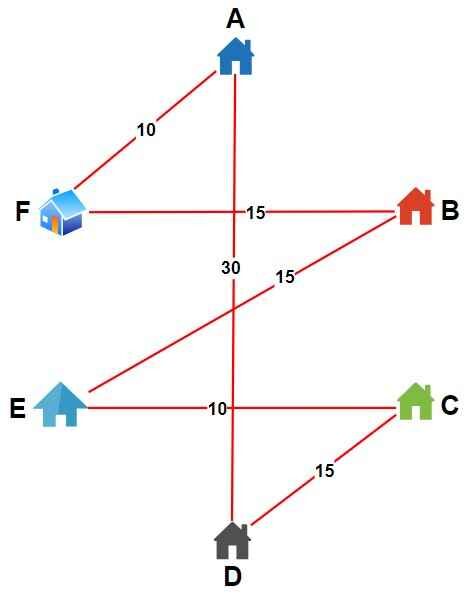
So, our tour is A → F → B → E → C → D → A
This solution demonstrates how the Nearest Neighbour Algorithm works and provides an approximate route based on local decisions at each step.
.
Source Code for Nearest Neighbour Problem
BOOKS