Held-Karp Algorithm for TSP

Distribute Education like Computer Geek

Introduction

.

The Held-Karp Algorithm or Traveling Salesman Problem (TSP) by Dynamic programming is a classic algorithmic problem in computer science and operations research.

The goal is simple – Given a list of cities and the distances between them, find the shortest possible route that visits each city exactly once and returns to the starting point.

This problem is crucial in fields like logistics, transportation, and manufacturing.

The TSP can be solved using various methods

  1. Brute Force – Check all possible routes and choose the shortest one. This method guarantees the optimal solution but is impractical for large datasets due to its high computational cost.
  2. Greedy Algorithms – Heuristics that make local optimal choices at each step to find a global optimum. It is also called Nearest Neighbour Problem.
  3. Dynamic Programming – Optimizes the problem by solving subproblems and combining their solutions. It is also called Held-Karp algorithm.
  4. Branch & Bound Approach – breaking the problem into smaller subproblems (branching) and calculating a lower bound for each subproblem. If the lower bound exceeds the current best solution, that branch is pruned (ignored).
  5. Approximation Algorithms – Provides near-optimal solutions in a reasonable time, useful for large instances. It is also called Christofides Algorithm.

We solve this problem by Greedy method and now we will solve the Travelling Salesman Problem by Dynamic Programming, and It is also called Held-Karp algorithm.

.

Held-Karp Algorithm

The Held-Karp algorithm, also known as the Dynamic Programming Solution for the Traveling Salesman Problem (TSP), is an exact algorithm that solves the TSP. It is named after Michael Held and Richard M. Karp, who introduced this approach in 1962.

Held-Karp algorithm is often referred to as the “Bellman-Held-Karp algorithm,” named after Richard Bellman, who developed the dynamic programming approach. Held and Karp adapted Bellman’s dynamic programming approach to efficiently solve the TSP, which led to the algorithm now known as the Bellman-Held-Karp algorithm.

.

Problem Statement

Given a set of n cities and a distance matrix that represents the distances between every pair of cities, the goal is to find the shortest possible route that:

  1. Starts at a specified city (or any city, since the problem is symmetric).
  2. Visits each city exactly once.
  3. Returns to the starting city.

.

AlgorithmforHeldKarp

Understanding the Problem

  • Imagine you have several cities and you want to find the shortest path that starts from one city, visits all other cities exactly once, and returns to the starting city.

Using Dynamic Programming

  • Instead of checking every possible route, which would be too slow, the Held-Karp algorithm breaks down the problem into smaller subproblems. It keeps track of the shortest paths to various subsets of cities and builds up to the solution.

State Representation

  • Define a state using two pieces of information:
    • Subset of Cities: A set of cities that have been visited so far.
    • Last City: The last city visited in this subset.

Dynamic Programming Table

  • Create a table (or use an array) where each entry dp[mask][i] represents the shortest path cost to visit all cities in the subset mask and end at city i. Here, mask is a bitmask representing which cities have been visited.

Initial State

  • Start with the initial city (often city 0) and initialize the table to reflect the cost of starting and ending at this city without visiting any others.

Transition Between States

  • To fill in the table, consider moving from one city to another. For each city i in a subset, compute the shortest path to each other city j not yet visited. Update the table with the minimum cost found.

Final Path Calculation

  • Once the table is fully populated, find the shortest route that visits all cities and returns to the starting city by examining the last entries in the table and adding the return cost to the starting city.

.

Example

Travelling Salesman Problem

.

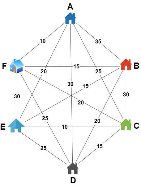
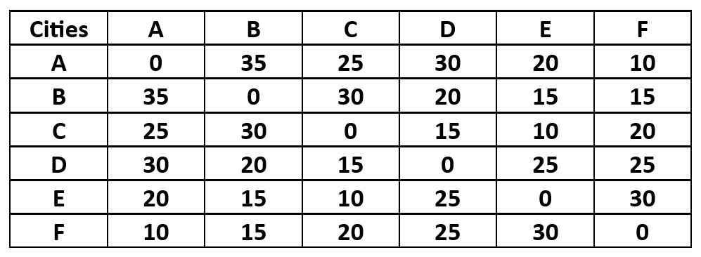
Example Distance Matrix

Travelling Salesman Problem adjacency matrix

.

Find a tour that visits each city exactly once and returns to the starting city by always moving to the nearest unvisited city.

.

Step 1 – Calculate the Minimum Cost Between Pairs of Cities

We begin by determining the direct travel costs between every pair of cities. These initial pairwise costs will be used as the base cases for our dynamic programming table.

  1. Cost from City A to City B (AB) is 35
  2. Cost from City A to City C (AC) is 25
  3. Cost from City A to City D (AD) is 30
  4. Cost from City A to City E (AE) is 20
  5. Cost from City A to City B (AF) is 10
  6. Cost from City B to City C (BC) is 30
  7. Cost from City B to City D (BD) is 20
  8. Cost from City B to City E (BE) is 15
  9. Cost from City B to City F (BF) is 15
  10. Cost from City C to City D (CD) is 15
  11. Cost from City C to City E (CE) is 10
  12. Cost from City C to City F (CF) is 20
  13. Cost from City D to City E (DE) is 25
  14. Cost from City D to City F (DF) is 25
  15. Cost from City E to City F (EF) is 30

There are 15 pairs of cities with costs ranging from 10 to 35. However, we do not find the minimum cost by simply choosing the smallest value among these pairs.

For example, if we pick the pair CE with a cost of 10, the remaining cities might require covering much larger distances, leading to a higher total cost. So, choosing just the smallest pair will not give us the optimal route that covers all cities at the lowest possible cost.

.

Then, what is the SOLUTION?

To find the optimal route, we don’t just stop at selecting the minimum cost between two cities. Instead, we must consider adding a third city to each of these pairs. This allows us to explore different routes and check how the total cost changes when we visit an additional city.

.

Step 2 –

1. Cost from City AB to third City.

  • Cost from City AB to City C ((AB)C) is 35+30 = 65
  • Cost from City AB to City D ((AB)D) is 35+20 = 55
  • Cost from City AB to City E ((AB)E) is 35+15 = 50
  • Cost from City AB to City F ((AB)F) is 35+15 = 50 

.

2. Cost from City AC to third City.

  • Cost from City AC to City B ((AC)B) is 25+30 = 50
  • Cost from City AC to City D ((AC)D) is 25+15 = 40
  • Cost from City AC to City E ((AC)E) is 25+10 = 35
  • Cost from City AC to City F ((AC)F) is 25+20 = 45 

.

3. Cost from City AD to third City.

…

…

…

15. Cost from City EF to third City.

  • Cost from City EF to City A ((EF)A) is 30+10 = 40
  • Cost from City EF to City B ((EF)B) is 30+15 = 45
  • Cost from City EF to City C ((EF)C) is 30+20 = 50
  • Cost from City EF to City D ((EF)D) is 30+25 = 55

In this step, when we add a third city to each pair, we end up calculating the cost 15*4 = 60 times.

When we add a fourth city, the number of calculations increases to 60*3 = 180 times.

Adding a fifth city leads to 180*2 = 360 calculations, and after that, we just need to add the sixth city and return to the starting city.

This process is very long and complex, which is why we typically solve it using a programming language.

In other dynamic programming problems, like matrix chain multiplication or subset sum, the DP table is relatively small. However, in the Traveling Salesman Problem, the table grows large very quickly, making manual calculations impractical. That’s why we rely on a programming language to compute the answer efficiently.

.

Using the programming language, we’ve successfully calculated the minimum cost for this 6-city example using the Held-Karp Algorithm. The total minimum cost for completing the tour is 90.

This result represents the lowest possible cost to visit all six cities exactly once and return to the starting city.

.

Source Code for Held-Karp Algorithm

Time Complexity of Held-Karp Algorithm

The time complexity of the Held-Karp algorithm for solving the Traveling Salesman Problem (TSP) is O(n2 * 2n), where n is the number of cities.

The algorithm computes the minimum cost for every subset of cities and for each subset, it considers every possible city to end the path. The total number of subsets is 2n, and for each subset, the algorithm performs O(n) operations, leading to a time complexity of O(n2 * 2n).

.

Space Complexity of Held-Karp Algorithm

The space complexity of the Held-Karp algorithm is O(n * 2n).

The algorithm uses a dynamic programming table, dp[subset][city], where subset represents the set of cities that have been visited and city represents the current city. There are 2n possible subsets, and for each subset, the algorithm stores a result for each of the n cities, leading to a space complexity of O(n * 2n).

.

Advantage of Held-Karp Algorithm
  1. It guarantees the optimal solution by exhaustively evaluating all possible tours.
  2. It uses dynamic programming to reduce redundant calculations, which is more efficient than brute-force methods.
  3. It provides a clear approach to solving TSP with a well-defined methodology.
  4. It systematically explores subsets of cities, ensuring that all possibilities are considered.
  5. It is particularly useful for small to medium-sized instances of the TSP where exact solutions are feasible.

.

Disadvantage of Held-Karp Algorithm
  1. Its time complexity is O(n2 * 2n), which grows exponentially with the number of cities, making it impractical for large instances.
  2. It requires O(n * 2n) space, which can be excessive for large problems.
  3. It is suitable only for small to medium-sized instances due to its computational and memory requirements.
  4. For large-scale TSP problems, it becomes infeasible to use due to the rapid growth in computational resources needed.
  5. The algorithm’s implementation can be complex and may require significant coding effort and debugging.

.

Application of Held-Karp Algorithm
  1. Optimization Problems – Solving TSP in logistics and routing to find the shortest possible route that visits a set of locations and returns to the origin.
  2. Network Design – Designing efficient network layouts and routing paths in telecommunications and computer networks.
  3. Operations Research – Applied in various operational scenarios where optimization of routes or schedules is crucial.
  4. Robotics – Used in path planning for robots to determine the most efficient path through a series of points.
  5. Supply Chain Management – Helps in optimizing delivery routes to minimize travel time and costs in supply chains.
  6. Scheduling – Assists in scheduling problems where tasks need to be executed in a specific order with minimal overall travel or transition time.

Test Yourself

Q1- Explain the main idea behind the Held-Karp algorithm for solving the TSP.

The Held-Karp algorithm uses dynamic programming to solve the TSP by breaking the problem into smaller subproblems. It keeps track of the shortest paths to various subsets of cities and builds up to the final solution.

The algorithm uses a bitmask to represent subsets of cities and updates the minimum cost of visiting each subset.

Q2- Compare the greedy algorithm and dynamic programming approach for TSP.

The greedy algorithm (Nearest Neighbour) makes local optimal choices at each step, which may not lead to the global optimum.

In contrast, the dynamic programming approach (Held-Karp algorithm) solves the problem optimally by considering all subsets of cities and their costs, though it has higher computational complexity compared to the greedy algorithm.

Q3- What is the time complexity of the Held-Karp algorithm and why?

The time complexity of the Held-Karp algorithm is O(n2 * 2n), where n is the number of cities.

This complexity arises because the algorithm evaluates all subsets of cities (2n) and performs operations involving each subset (n2), leading to a substantial computational cost for large n.

Q4- Why is the Held-Karp algorithm more suitable for smaller instances of TSP?

The Held-Karp algorithm is more suitable for smaller instances because its time complexity grows exponentially with the number of cities.

For larger instances, the number of calculations becomes impractical, making it challenging to compute the optimal solution within a reasonable time frame.

Q5- Compare the Brute Force method and the Dynamic Programming approach for solving the Traveling Salesman Problem (TSP).

Brute Force algorithm

The Brute Force algorithm for solving the Traveling Salesman Problem (TSP) involves generating and evaluating all possible permutations of the cities to determine the shortest possible tour. It calculates the total distance for every permutation and selects the one with the minimum distance as the optimal solution.

Its time complexity is O((n-1)!), where n is the number of cities. This factorial growth makes it impractical for large datasets.

Limitations

  • Computationally infeasible for large numbers of cities due to its factorial time complexity.
  • Requires evaluating an extremely large number of permutations.

Held-Karp algorithm

The Held-Karp algorithm is a dynamic programming approach for solving the Traveling Salesman Problem (TSP). It breaks down the problem into smaller subproblems and uses a bitmask to represent subsets of cities. The algorithm iteratively builds up the solution by combining the results of subproblems to find the shortest path that visits all cities.

The time complexity of the Held-Karp algorithm is O(n2 * 2n), where n is the number of cities.

Limitations

  • Still suffers from exponential time complexity, making it impractical for very large datasets.
  • High space complexity as it needs to store intermediate results for all subsets of cities.
Q6- In the Held-Karp algorithm, what does the DP table entry dp[mask][i] represent?
  1. Cost of the shortest path from city i to city 0
  2. Cost of visiting all cities in subset mask and ending at city i
  3. Cost of visiting all cities from city 0 to city i
  4. Cost of traveling from city i to all other cities

Ans – (2)

Explanation – The DP table entry dp[mask][i] represents the minimum cost of visiting all cities in the subset mask and ending at city i.

Q7- What is the primary advantage of using dynamic programming for TSP compared to greedy algorithms?
  1. Simplicity
  2. Speed
  3. Optimality
  4. Low memory usage

Ans – (3)

Explanation – Dynamic programming provides an optimal solution by considering all subsets and transitions, whereas greedy algorithms may not always find the global optimum.

Q8- Which approach involves calculating a lower bound for subproblems and pruning branches that cannot lead to an optimal solution?
  1. Brute Force
  2. Greedy Algorithms
  3. Branch and Bound
  4. Approximation Algorithms

Ans – (3)

Explanation – The branch and bound approach involve calculating a lower bound and pruning branches to reduce the number of solutions explored.

Q9- Which of the following algorithms is known for providing a guaranteed approximation within 3/2 of the optimal solution for TSP?
  1. Nearest Neighbour Algorithm
  2. Held-Karp Algorithm
  3. Christofides Algorithm
  4. Brute Force Algorithm

Ans – (3)

Explanation – The Christofides Algorithm provides a solution that is guaranteed to be within 3/2 times the optimal solution for the TSP.

Q10- What is the primary disadvantage of using the Dynamic Programming approach for solving TSP?
  1. Inability to find the optimal solution
  2. High space complexity
  3. High computational time for small datasets
  4. Lack of efficiency for heuristic solutions

Ans – (2)

Explanation – The primary disadvantage of the Dynamic Programming approach is its high space complexity, as it requires storing results for all subsets of cities.

Q11- What does the term ‘subproblem’ refer to in the context of the Held-Karp algorithm?
  1. The distance between two cities
  2. A smaller part of the overall TSP problem
  3. The final tour path
  4. A heuristic solution

Ans – (2)

Explanation – In the Held-Karp algorithm, a ‘subproblem’ refers to solving smaller instances of the TSP problem, which are then combined to find the solution to the overall problem.

BOOKS

Algorithm T H CoremanAlgorithm by Udit AgarwalAlgorithm Ellis HorowitzData Structure & Algorithm Made Easy Narasimha

Â