

Introduction to Depth First Search Algorithm
.
Depth First Search (DFS) is a fundamental algorithm used in the field of computer science, specifically in the design and analysis of algorithms.
It is primarily employed for traversing or searching tree or graph data structures.
DFS explores as far as possible along each branch before backtracking, making it particularly useful for solving problems involving interconnected nodes.
.
History
DFS originated from maze-solving techniques by Charles Pierre Trémaux in the 19th century. Formalized by Charles Leonard Hamblin in 1954, it recursively explores graph/tree structures.
DFS gained prominence in the 1960s, becoming fundamental in graph theory and various applications like network analysis and AI.
Trémaux and Hamblin’s contributions paved the way for DFS as a crucial algorithm in computer science.
They proposed a method for solving mazes by consistently following either the left-hand or right-hand rule.
By adhering to this rule, where you always turn in the same direction (left or right) at every junction, it becomes possible to navigate through the maze and eventually reach the exit. This approach simplifies the maze-solving process and provides a systematic way to explore and solve maze puzzles.
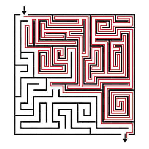
It follows the left-hand rule and with this method we come out from exit.
In solving this maze, we follow left hand rule of Depth First Search (DFS) Algorithm, but here it is not the complete DFS. I tell you why
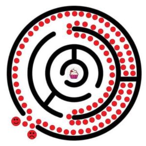
In this maze, we follow the left-hand rule and we could not even reach the cupcake in the innermost circle. That’s why it’s not DFS because DFS will cover all the remaining points in the graph, including the cupcake.
.
Definition
- Basic Principle – It starts at a selected node (often referred to as the “root“) and explores as far as possible along each branch

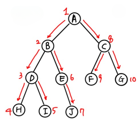
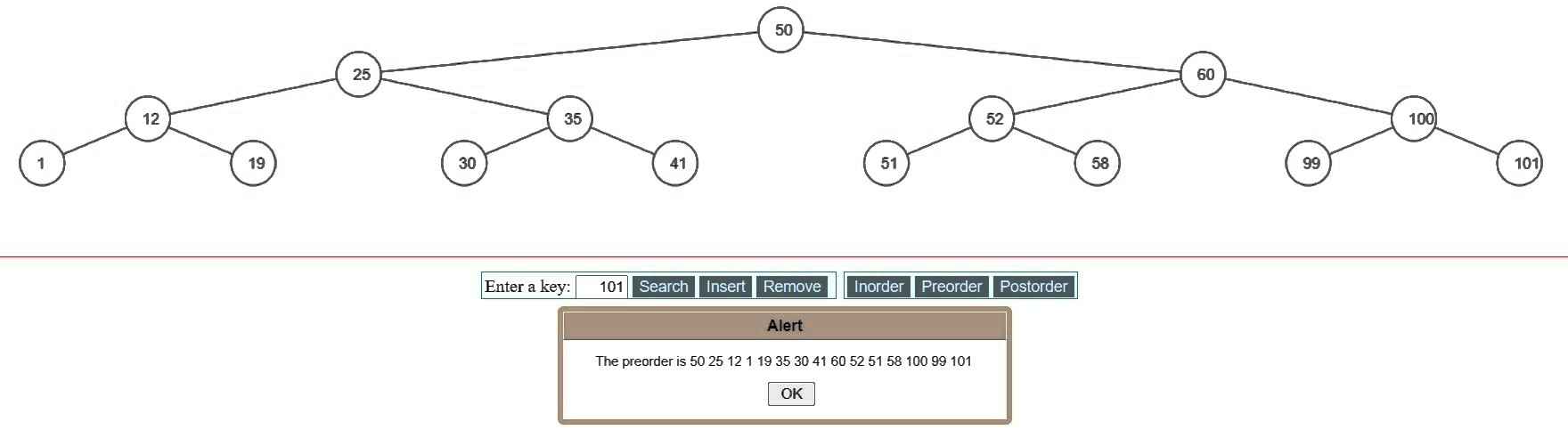
- Depth First Search (DFS) can be likened to a preorder traversal of a tree. In a preorder traversal, the algorithm starts from the root node and visits each node’s subtree recursively in a depth-first manner. Similarly, in DFS, the algorithm explores as far as possible along each branch before backtracking, effectively traversing the entire graph or tree structure in a depth-first manner.
.
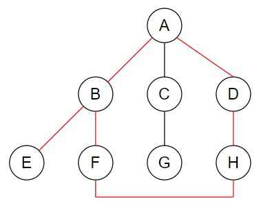
- DFS keeps track of previously visited nodes using timestamps to prevent infinite loops or non-termination. If the search is conducted without keeping track of previously visited nodes, it will visit the nodes in the following order: A, B, E, F, H D, A, B, E, F, H, etc. This will keep the user stuck in the A, B, E, F, H, D cycle and prevent them from ever reaching C and G.
- Each vertex has two timestamps – 1. Discovery Timestamp d[v] 2. Finishing Timestamp f[v], and for every vertex, its discovery timestamp < finishing timestamp.
- Recursive Nature – DFS employs recursion or a stack-based approach to traverse the graph, visiting adjacent unvisited nodes until all nodes are visited or a specific condition is met.
.
Algorithm of DFS
- Initialization:
- Create a stack to store vertices.
- Initialize all vertices as undiscovered (white).
- DFS Algorithm:
- Start from a chosen vertex and mark it as discovered (gray).
- Push the vertex onto the stack.
- While the stack is not empty
- Peek at the top vertex of the stack.
- If the vertex has undiscovered neighbors
- Choose an undiscovered neighbor.
- Mark the neighbor as discovered (gray) and push it onto the stack.
- If the vertex has no undiscovered neighbors or all neighbors are visited
- Pop the vertex from the stack.
- Mark the vertex as finished (black).
- Repeat until all vertices are visited.
- Recording Discovery and Finishing Times
- Initialize a global timestamp variable.
- When a vertex is discovered, record its discovery time as the current timestamp.
- When a vertex is finished, record its finishing time as the current timestamp.
- Increment the timestamp after each discovery or finishing event.
- Backtracking
- After DFS traversal completes, if needed for specific applications, backtrack through the graph to find paths or perform additional operations.
.
Example
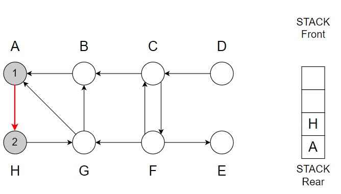
Step 1 – Start from vertex A.
Color of A = Grey
Discover time = 1
Vertex A is top of the Stack.

Step 2 – A -> H
Color of H = Grey
Discover time = 2
Vertex H is top of the Stack.
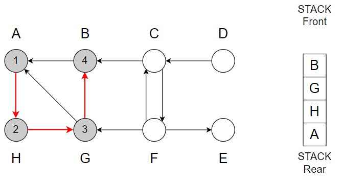
Step 3 – H -> G
Color of G = Grey
Discover time = 3
Vertex G is top of the Stack.

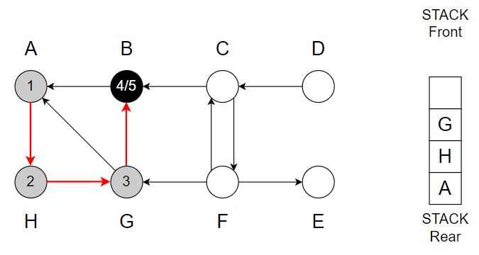
Step 4 – G -> B
Color of B = Grey
Discover time = 4
Vertex B is top of the Stack.
Step 5 – B -> only A (A is already in the Stack)
Pop B from the Stack
Color of B = Black
Finishing time = 5 and backtrack.
Vertex G is top of the Stack.
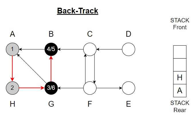
Step 6 – B <- G (G -> A and A is already in the Stack)
Pop G from the Stack
Color of G = Black
Finishing time = 6 and backtrack.
Vertex H is top of the Stack.
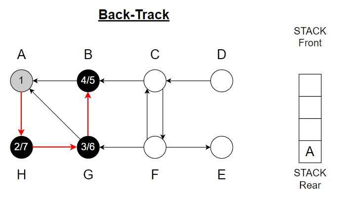
Step 7 – G <- H
Pop H from the Stack
Color of H = Black
Finishing time = 7 and backtrack.
Vertex A is top of the Stack.
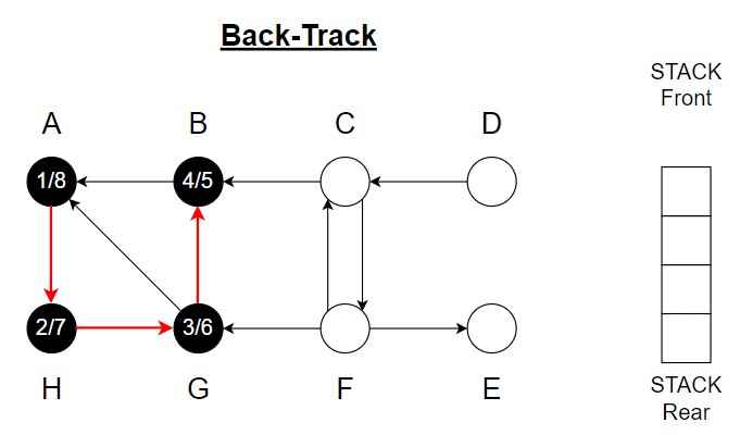
Step 8 – H -> A
Pop A from the Stack
Color of A = Black
Finishing time = 8.
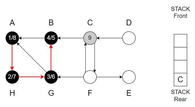
Stack is empty.
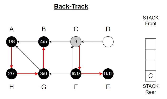
Step 9 – Choose vertex C.
Color of C = Grey
Discover time = 9
Vertex C is top of the Stack.
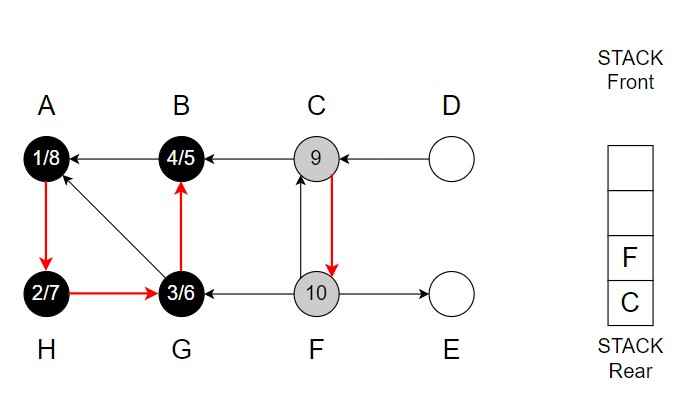
Step 10 – C -> F
Color of F = Grey
Discover time = 10
Vertex F is top of the Stack.
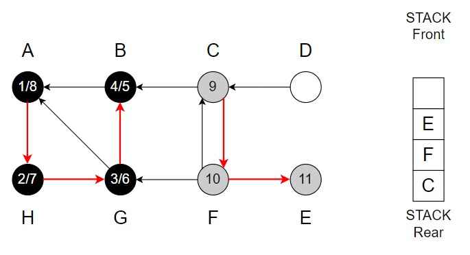
Step 11 – F -> E
Color of E = Grey
Discover time = 11
Vertex E is top of the Stack.
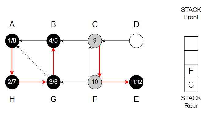
Step 12 – E has no adjacent vertex.
Pop E from the Stack.
Color of E = Black
Finishing time = 12 and backtrack.
Vertex F is top of the Stack.
Step 13 – E <- F
Pop F from the Stack.
Color of F = Black
Finishing time = 13
Vertex C is top of the Stack.
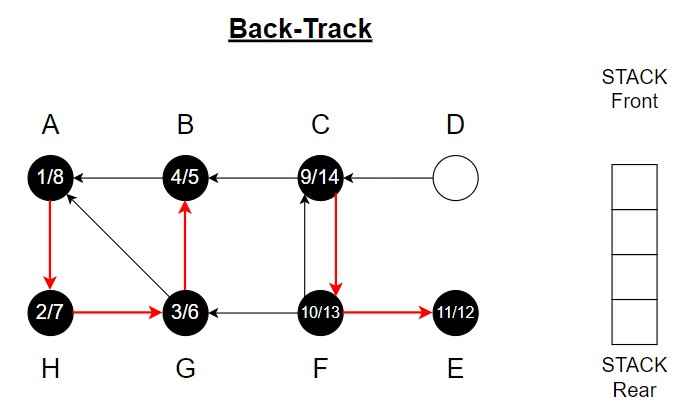
Step 14 – F <- C
Pop C from the Stack.
Color of C = Black
Finishing time = 14
Stack is empty.
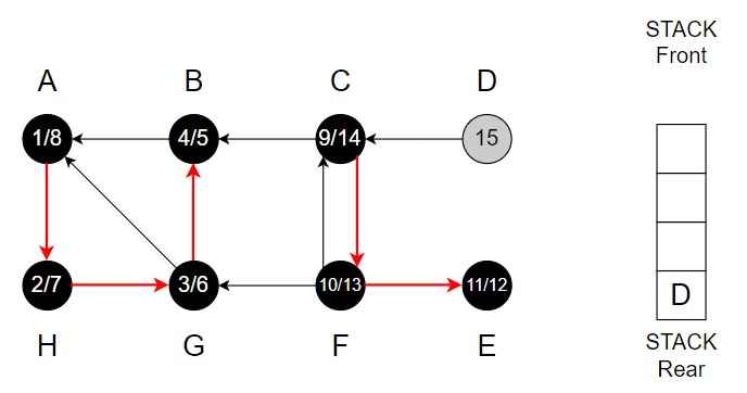
Step 15 – Choose vertex D.
Color of D = Grey
Discover time = 15
Vertex D is top of the Stack.
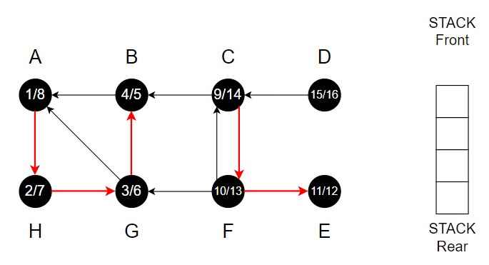
Step 16 – D has adjacent vertex C and C is already black.
Pop D from the Stack.
Color of D = Black
Finishing time = 16
Stack is empty.
.
Source Code of Depth First Search
BOOKS