

Introduction to Bellman-Ford Algorithm
.
The Bellman-Ford algorithm is a fundamental method used in the design and analysis of algorithms.
“It is particularly useful for finding the shortest paths from a single source vertex to all other vertices in a weighted graph, even in the presence of negative weight edges, making it a versatile tool in various applications.”
Bellman-Ford is more versatile as it can handle graphs with negative weight edges and detect negative weight cycles.
.
Bellman-Ford Algorithm Vs. Dijkstra’s Algorithm
Criteria | Bellman-Ford Algorithm | Dijkstra’s Algorithm |
Single Source Shortest Paths | Finds shortest paths from a single source to all other vertices, even with negative weight edges. | Finds shortest paths from a single source to all other vertices, but assumes non-negative weights. |
Time Complexity | O(V * E) | O((V + E) * log(V)) |
Space Complexity | O(V) | O(V + E) |
Negative Weight Edges | Handles graphs with negative weight edges. | Assumes non-negative weights; may produce incorrect results in the presence of negative weights. |
Performance | Slower in general, especially for dense graphs or graphs with negative weight edges. | Faster, particularly in graphs with non-negative weights. |
Optimizations | Can be optimized for certain cases, such as early stopping if no relaxation occurs in an iteration. | Efficient with data structures like priority queues, allowing for quicker updates of distances. |
Use Cases | Suitable for graphs with negative weight edges, where Dijkstra’s algorithm may fail. | Preferred for graphs with non-negative weights due to its efficiency. |
Negative Weight Cycles | Can detect negative weight cycles in the graph. | Does not detect negative weight cycles. |
.
History
The Bellman-Ford algorithm, named after its inventors Richard Bellman and Lester Ford, both were American mathematician and computer scientist, has its roots in the field of operations research and computer science.

The algorithm builds upon foundational concepts in graph theory, which dates back to the 18th century with the work of mathematicians like Leonhard Euler. Euler’s solution to the Seven Bridges of Königsberg problem laid the groundwork for graph theory, which became a fundamental area of study in mathematics and computer science.
Richard Bellman, introduced the concept of dynamic programming in the 1950s. In collaboration with Lester Ford, Bellman extended these ideas to develop an algorithm for solving the single-source shortest path problem in a graph with both positive and negative edge weights.
.
Negative – weight Edges
Negative weight edges in a graph are edges that have weights assigned to them, and these weights are less than zero.
In simpler terms, when you’re looking at a graph where the edges represent connections between points, a negative weight edge means that it gained by you something to traverse that edge.
For example, in a map where cities are represented by points and roads between them by edges, a negative weight edge might signify a road where you gain money or save time by traveling along it. This is contrary to a regular edge where you typically spend time or money to travel along it.
.
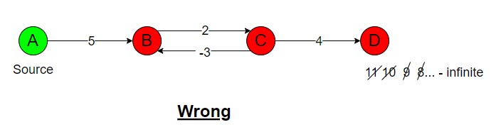
Negative Cycles
Negative weight edges can complicate finding the shortest path in a graph. If there are no negative weight cycles reachable from the starting point, the shortest path remains clear even if it has negative values.
However, if such cycles exist, defining the shortest path becomes unclear. If a negative weight is encountered along the path, it’s labelled as negative infinity, indicating ambiguity in defining the shortest path.
Note – Both Dijkstra’s algorithm and the Bellman-Ford algorithm are versatile and can be used effectively in both directed and undirected graphs to find shortest paths.
.
Algorithm of Bellman-Ford
G – Weighted graph represented as an adjacency list or matrix.
Source – The source vertex from which shortest paths are calculated.
Initialization
- Create an array dist[] of size V (number of vertices in G) to store the shortest distance from the source vertex to each vertex.
- Initialize dist[source] = 0 and dist[v] = Infinity for all other vertices v.
Main Algorithm
- Repeat the following step V – 1 times (where V is the number of vertices in the graph).
- For each edge (u, v) in the graph, relax the edge.
- If dist[u] + weight(u, v) < dist[v], update dist[v] = dist[u] + weight(u, v) and set prev[v] = u.
- After V – 1 iterations, all shortest paths from the source vertex are found unless there are negative weight cycles.
Check for Negative Cycles
- Iterate over all edges (u, v) in the graph and check if there is any improvement in dist[v] by relaxing the edge (u, v).
- If dist[u] + weight(u, v) < dist[v], then there exists a negative weight cycle reachable from the source vertex.
Optionally, you can perform an additional step to trace back and identify the vertices in the negative weight cycle.
.
Example

.
Now, let’s apply the Bellman-Ford algorithm with source vertex A.
Initialization
Initialize dist[] array
dist[] = {0, ∞, ∞, ∞, ∞, ∞}

.
Perform relaxation
V = {A, B, C, D, E, F} in this graph. So, to get the shortest distance in vertex, the edges need to relax V – 1 times (5 times).
Relaxation refers to the process of updating the shortest distance estimate to a vertex if a shorter path to that vertex is discovered.
The edges are (A, B), (A, F), (F, E), (B, F), (B, C), (B, E), (C, E), (C, D), (E, D).
Step by step check all the edges and write the shortest weight in vertices by applying a formula
Formula is, dist[v] = min(dist[v], dist[u] + weight(u, v))
.
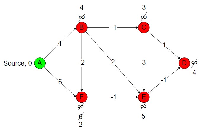
Iteration 1
.
For (A, B), dist[B] = min(∞, 0 + 4) = 4
For (A, F), dist[F] = min(∞, 0 + 6) = 6
For (F, E), dist[E] = min(∞, 6 – 1) = 5
For (B, F), dist[F] = min(6, 4 – 2) = 2
For (B, C), dist[C] = min(∞, 4 – 1) = 3
For (B, E), dist[E] = min(5, 4 + 2) = 5
For (C, E), dist[E] = min(5, 3 + 3) = 5
For (C, D), dist[D] = min(∞, 3 + 1) = 4
For (E, D), dist[D] = min(∞, 5 – 1) = 4
.
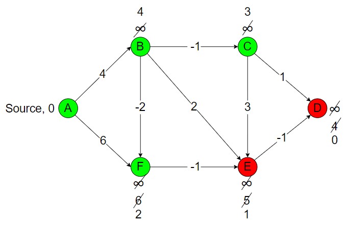
Iteration 2
.
For (A, B), dist[B] = min(4, 0 + 4) = 4
For (A, F), dist[F] = min(2, 0 + 6) = 2
For (F, E), dist[E] = min(5, 2 – 1) = 1
For (B, F), dist[F] = min(2, 4 – 2) = 2
For (B, C), dist[C] = min(3, 4 – 1) = 3
For (B, E), dist[E] = min(1, 4 + 2) = 1
For (C, E), dist[E] = min(1, 3 + 3) = 1
For (C, D), dist[D] = min(4, 3 + 1) = 4
For (E, D), dist[D] = min(4, 1 – 1) = 0
Check for negative weight cycles
Relax all edges one more time.
Iteration 3

.
For (A, B), dist[B] = min(4, 0 + 4) = 4
For (A, F), dist[F] = min(2, 0 + 6) = 2
For (F, E), dist[E] = min(5, 2 – 1) = 1
For (B, F), dist[F] = min(2, 4 – 2) = 2
For (B, C), dist[C] = min(3, 4 – 1) = 3
For (B, E), dist[E] = min(1, 4 + 2) = 1
For (C, E), dist[E] = min(1, 3 + 3) = 1
For (C, D), dist[D] = min(4, 3 + 1) = 4
For (E, D), dist[D] = min(4, 1 – 1) = 0
In iteration 3, No changes in dist[], so no negative weight cycles detected.
After the Bellman-Ford algorithm completes, the shortest distances from vertex A to all other vertices are
A = 0
B = 4,
C = 3,
D = 0,
E = 1,
F = 2.
Source Code of Bellman Ford Algorithm
BOOKS