Collision Handling
(Open Addressing)

Collision Handling Technique – Open Addressing

Imagine a classroom with fixed chairs. A student comes in. His seat number is 7. But seat 7 is already occupied. Now what?

In Separate Chaining, we add another chair beside it.

But in Open Addressing, we do something different. We say – “Find another empty seat inside the same classroom.” That is the core idea of Open Addressing in hashing.

Today, we will understand Open Addressing clearly – its types, algorithms, examples, time complexity, space complexity, and real applications. If you are preparing for GATE, UGC NET, placements, or interviews, this topic is extremely important.

.

What is Open Addressing?

Open Addressing is a collision handling technique in hashing where –

• All elements are stored inside the hash table array itself.
• If collision happens, we probe (search) for another empty slot using a specific probing technique.

No linked lists. No extra memory. Just smart searching. In this technique, load factor α must always be less than 1. Because once the table is full, insertion stops.

.

Types of Open Addressing

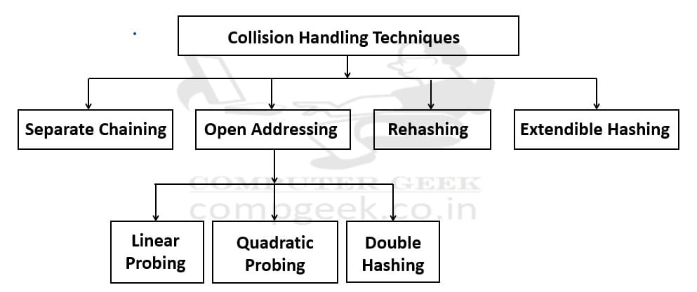
There are three main searching (probing) techniques –

1. Linear Probing
2. Quadratic Probing
3. Double Hashing

Each one tries to solve collision in a slightly smarter way.

1. Linear Probing

“If collision occurs at index h(k), check the next index. If that is full, check the next. Continue until an empty slot is found.”

Simple. Straight. Like standing in a queue.

.

Algorithm – Linear Probing

Insertion –

1. Compute index = h(k)
2. If slot is empty, insert
3. Else check (index + 1) mod m
4. Repeat until empty slot found

Searching –

1. Compute index = h(k)
2. If key found, return
3. Else check next slot
4. Stop when empty slot found or key located

Example

Let m = 7 and Hash function h(k) = k mod 7

Insert keys – 10, 17, 24

10 mod 7 = 3 → index 3^rd is empty → insert 10.
17 mod 7 = 3 → collision → check 4^th index (empty) → insert 17
24 mod 7 = 3 → collision → check 4^th index (full) → check 5^th Index (empty) → insert 24

Table looks like –

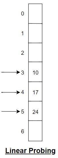
You see a cluster forming. This is called Primary Clustering.

Time Complexity – Linear Probing

• Best case – O(1)
• Average case – O(1) when α small
• Worst case – O(n)

As load factor increases, clusters grow. Performance degrades sharply.

Space Complexity – Linear Probing

The space complexity of Linear probing is O(m). There is no extra linked lists. It is only an array.

.

2. Quadratic Probing

“In open addressing, when collision happens, we must find another empty place inside the same hash table. In quadratic probing, we do not move step by step. We move in square steps.”

Suppose a key is hashed to index h(k), and that position is already full. Then we check –

h(k) + 1²
h(k) + 2²
h(k) + 3²
and so on (mod m)

So actually we are jumping like +1, +4, +9, +16 …

Because of this square movement, elements do not form a long continuous cluster like in linear probing. They get more space and spread better inside the table.

In simple words, quadratic probing handles collision by checking positions at increasing square distances instead of checking every next index. It reduces clustering, but it still cannot remove it completely.

.

Algorithm – Quadratic Probing

Insertion –

1. Compute h(k)
2. For i = 0 to m-1:
   index = (h(k) + i²) mod m
3. Insert at first empty slot

Searching –

Same probing sequence used until key found or empty slot encountered.

1. Compute index = h(k)
2. If key found, return
3. Else check next slot
4. Stop when empty slot found or key located

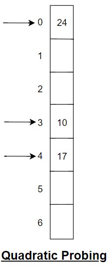
Example

Let m = 7 and H(k) = k mod 7

Insert – 10, 17, 24

10 mod 7 = 3 → index 3^rd is empty → insert 10.
17 mod 7 = 3 → collision → 3 + 1² = 4 → index 4^th is empty → insert 17
24 → collision → 3 + 1² = 4 (full) → 3 + 2² = 7 mod 7 = 0 → index 0^th is empty → insert 24

Now keys are more spread out.

Table looks like –

Time Complexity – Quadratic Probing

• Best case – O(1)
• Average case – O(1) when α small
• Worst case – O(n)

It reduces primary clustering but still has Secondary Clustering. Keys with same initial hash follow same probe sequence

Space Complexity – Quadratic Probing

The space complexity of Quadratic probing is O(m). There is no extra linked lists. It is only an array.

.

3. Double Hashing

“In open addressing, when collision happens, we must search for another empty position inside the same hash table, we use one more hash function to decide how far we should jump.”

If collision happens at h1(k), then the next position is calculated as –

h1(k) + i × h2(k) (mod m) where i = 0 to m-1.

Here, h2(k) = k mod p, where p is equal to the prime number less than m.

.

So, h2(k) gives the jump value, and this jump value is different for different keys.

Because the step size depends on the key itself, keys do not follow the same probing pattern. So clustering is reduced a lot compared to linear and quadratic probing.

.

Algorithm – Double Hashing

Insertion –

1. Compute h1(k)
2. Compute h2(k)
3. For i = 0 to m-1:
   index = (h1(k) + i × h2(k)) mod m
4. Insert at first empty slot

Searching –

Follow same probing sequence.

1. Compute index = h(k)
2. If key found, return
3. Else check next slot
4. Stop when empty slot found or key located

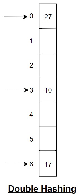
Example

Let m = 7 and Hash function h1(k) = k mod 7
h2(k) = i + (k mod 5) (i = 0 to m-1 & p = 5 less than m)

Insert key – 10, 17, 24

10 mod 7 = 3 → index 3^rd is empty → insert 10.

17 mod 7 = 3 → collision → (h1(k) + (i*(h2(k)))) mod 7
This is equal to – (3 + (1*(17 mod 5))) mod 7 = (3 + 2) mod 7 = 5^th index (empty) → insert 17.

24 mod 7 = 3 → collision → (h1(k) + (i*(h2(k)))) mod 7
This is equal to – (3 + (2*(17 mod 5))) mod 7 = (3 + 4) mod 7 = 0^th index (empty) → insert 24.

Table looks like –

Time Complexity – Double Hashing

• Best case – O(1)
• Average case – O(1)
• Worst case – O(n)

Among all open addressing methods, double hashing gives best distribution.

Space Complexity – Double Hashing

The space complexity of Double Hashing is O(m). There is no extra linked lists. It is only an array.

.

Comparison

Linear Probing

• Simple
• Suffers from primary clustering

Quadratic Probing

• Reduces primary clustering
• Still secondary clustering

Double Hashing

• Best distribution
• Least clustering

But all require α < 1. As α approaches 1, performance collapses.

.

Applications of Open Addressing

Open Addressing is used in

• Hash tables in embedded systems
• Memory-constrained environments
• Symbol tables in compilers
• High-performance in-memory caches