Dijkstra's Algorithm

Distribute Education like Computer Geek

Understanding Dijkstra’s Algorithm

Introduction

Dijkstra’s algorithm is a fundamental concept in the field of computer science, specifically in the realm of algorithm design and analysis.

It is named after the Dutch computer scientist Edsger W. Dijkstra, who introduced it in 1956 and three years later published.

This algorithm is widely used for finding the shortest path between nodes in a graph, especially in scenarios where the graph contains non-negative weights on its edges.

.

How It Works

Dijkstra’s algorithm works by iteratively exploring nodes in a graph, gradually building up the shortest paths from a designated source node to all other nodes.

.

History of Dijkstra’s Algorithm

When working as a programmer at the Mathematical Centre in Amsterdam in 1956, Dijkstra considered the shortest path issue in order to illustrate the capabilities of a new computer known as ARMAC.

His goal was to select both a problem and a solution (generated by a computer) that non-computer users could understand.

He created the shortest path algorithm and later implemented it for ARMAC, which used it to create a somewhat simplified transport map of 64 Dutch cities (6 bits would be sufficient to encode the city number).

Edsger W. Dijkstra independently developed an algorithm similar to Prim’s minimum spanning tree algorithm, which was initially discovered by Zernike and later rediscovered by Prim. Dijkstra’s publication of the algorithm occurred in 1959, coming two years after Prim’s and 29 years subsequent to Zernike’s discovery.

.

Algorithm of Dijkstra’s Sort
  1. Initialization
    • Assign a source node from which the shortest paths will be calculated.
    • Create a set to keep track of visited nodes.
    • Initialize an array or data structure to store the shortest distances from the source to each node.
    • Set the distance of the source node to 0 and all other nodes to infinity.
  1. Iteration
    • While there are unvisited nodes
    • Select the unvisited node with the smallest known distance as the current node.
    • Mark the current node as visited.
  1. Update Distances
    • For each neighbouring node of the current node that is still unvisited,
    • Calculate the tentative distance from the source to the neighbouring node through the current node.
    • If the tentative distance is shorter than the current known distance to that neighbouring node, update the distance.
  1. Repeat
    • Repeat steps 2 and 3 until all nodes are visited or the destination node is reached.


  1. Result
    • Once the algorithm completes, the array or data structure containing the shortest distances will provide the shortest path from the source node to all other nodes in the graph.

.

Example

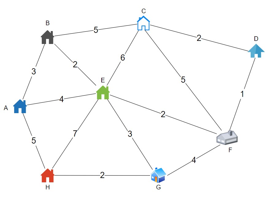
Let’s consider a road network represented as a graph where cities are the nodes and roads between cities are the edges. We’ll use Dijkstra’s algorithm to find the shortest path from a source city to a destination city.

The following graph displays the houses P, Q, R, S, T, U, V, and W as vertices, and the roads connecting them as edges. The time, expressed in hours, that the car takes to drive between each house is indicated by the numbers on the sides.

Dijkstra's Algorithm Graph

.

Step 1 – Start at the source node (let’s say A) with distance 0 and all other nodes to infinity.
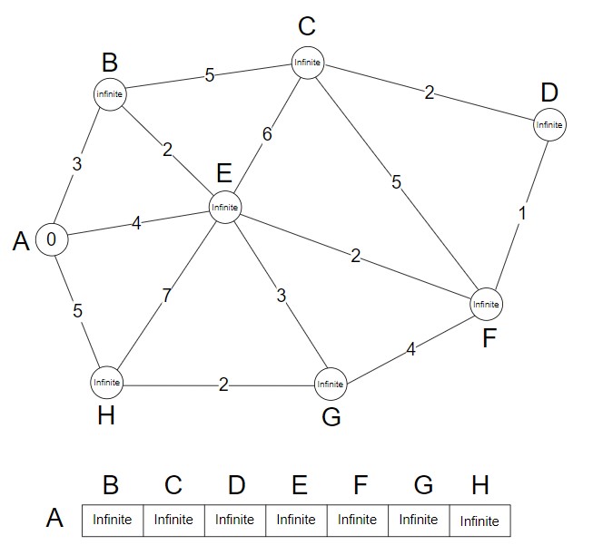
Dijkstra's Algorithm Graph

.

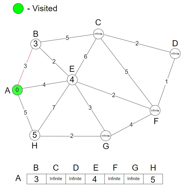
Step 2 – We mark the node A as visited.

A —> B, Cost of AB is 3, (Shortest Distance)

A —> E, Cost of AE is 4

A —> H, Cost of AH is 5

We have to find the minimum cost. So, we update the shortest distance (AB, 3).


Dijkstra's Algorithm Step 2

.

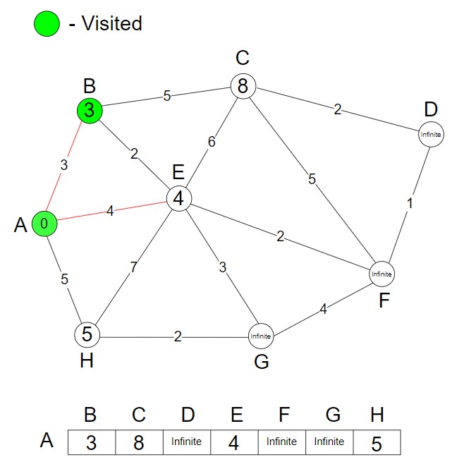
Step 3 – We mark the node B as visited.

A —> B —> C, Cost of ABC is 8

A —> B —> E, Cost of ABE is 5

A —> E, Cost of AE is 4, (Shortest Distance)

A —> H, Cost of AH is 5

We have to find the minimum cost. So, we update the shortest distance (AE, 4).

Dijkstra's Algorithm Step 3

.

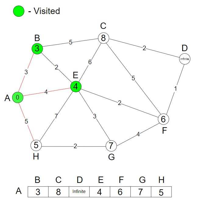
Step 4 – We mark the node E as visited.
A —> B —> C, Cost of AC is 8
A —> E —> F, Cost of AEF is 6
A —> E —> G, Cost of AEG is 7
A —> H, Cost of AH is 5, (Shortest Distance)
We have to find the minimum cost. So, we update the shortest distance (AH, 5).

Dijkstra's Algorithm Step 4

.

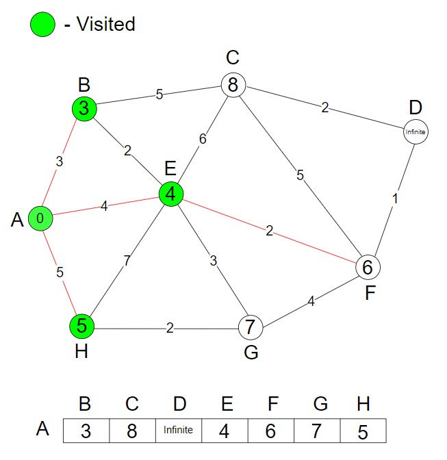
Step 5 – We mark the node H as visited.

A —> B —> C, Cost of AC is 8

A —> E —> F, Cost of AEF is 6, (Shortest Distance)

A —> E —> G, Cost of AEG is 7

A —> H —> G, Cost of AHG is 7

We have to find the minimum cost. So, we update the shortest distance (AEF, 6).

Dijkstra's Algorithm Step 5

.

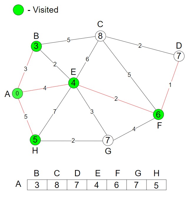
Step 6 – We mark the node F as visited.

A —> B —> C, Cost of AC is 8

A —> E —> F —> D, Cost of AEFD is 7, (Shortest Distance)

A —> E —> G, Cost of AEG is 7

A —> H —> G, Cost of AHG is 7

We have to find the minimum cost. So, we update the shortest distance (AEFD, 7).

Dijkstra's Algorithm Step 6

.

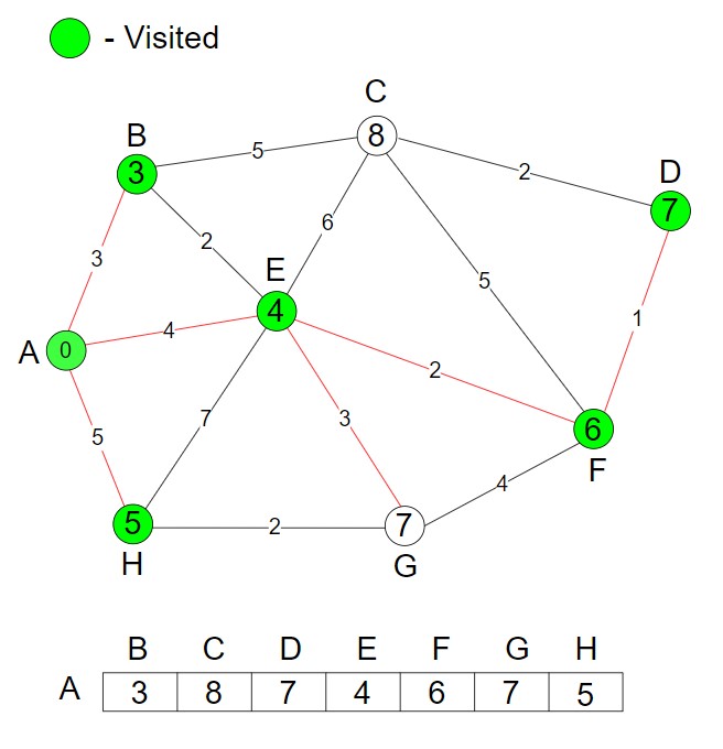
Step 7 – We mark the node D as visited.

A —> B —> C, Cost of AC is 8

A —> E —> G, Cost of AEG is 7, (Shortest Distance)

A —> H —> G, Cost of AHG is 7

We have to find the minimum cost. So, we update the shortest distance (AEG, 7).

Dijkstra's Algorithm Step 7

.

Step 8 – We mark the node G as visited.

A —> B —> C, Cost of AC is 8, (Shortest Distance)

We have to find the minimum cost. So, we update the shortest distance (ABC, 8).

Also, mark the node C as visited.

Dijkstra's Algorithm Step 8

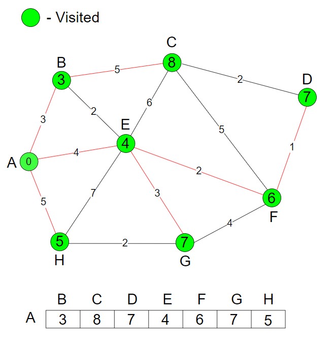
Dijkstra’s Algorithm is complete.

.

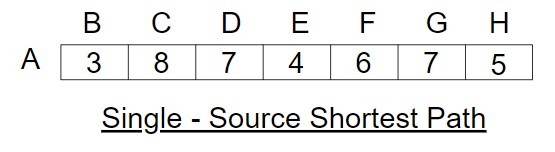
Note – I have just solved an array which has the shortest distance from source node A to the remaining vertices. This is the single source shortest path which we have come across now.

Single - Source Shortest Path

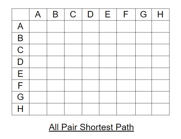
If I declare all the vertices as source nodes and find the shortest path of all the vertices then I use All pair shortest path.

All Pair Shortest Path

.

Source Code of Dijkstra’s Algorithm

Time Complexity of Dijkstra’s Algorithm

The time complexity of Dijkstra’s algorithm depends on the data structures used to implement it. Here’s a breakdown of the time complexity:

  1. Using an adjacency matrix

   – If the graph has V vertices and E edges, selecting the vertex with the minimum distance takes O(V) time.

   – Updating the distances of adjacent vertices takes O(V) time for each vertex.

   – Overall, the time complexity of the algorithm using an adjacency matrix is O(V2).


  1. Using a priority queue (min-heap)

   – With a binary heap or Fibonacci heap as the priority queue, selecting the vertex with the minimum distance takes O(log V) time.

   – Updating the distances of adjacent vertices takes O(log V) time for each vertex.

   – Considering that each edge is processed once, the total time complexity becomes O((V + E)log V).

.

Space Complexity of Dijkstra’s Algorithm

The space complexity of Dijkstra’s algorithm is O(V), where V is the number of vertices in the graph.

This space is primarily used for maintaining data structures like priority queues and distance arrays.

.

Advantages of Dijkstra’s Algorithm

– Finds the shortest path from a single source to all other vertices in a non-negative weighted graph.

– Efficient and widely applicable in various scenarios, such as network routing algorithms and GPS navigation systems.

.

Disadvantages of Dijkstra’s Algorithm

– Limited to graphs with non-negative edge weights.

– Inefficient for graphs with negative edge weights or cycles.

– Requires additional data structures like priority queues, which can increase space complexity.

.

Applications of Dijkstra’s Algorithm

– Network routing protocols in computer networks.

– GPS navigation systems for finding the shortest routes.

– Traffic management systems for optimizing travel paths.

– Shortest path algorithms in transportation and logistics.

Test Yourself

Q1- Explain Dijkstra’s algorithm and its significance in graph theory.

Dijkstra’s algorithm is a method for finding the shortest paths between nodes in a graph, especially in scenarios where all edge weights are non-negative. It explores nodes in a graph iteratively, gradually building up the shortest paths from a designated source node to all other nodes. This algorithm is significant because it has various practical applications in network routing, GPS navigation, and traffic management systems, among others.

Q2- Discuss the difference between Dijkstra’s algorithm and Prim’s algorithm.

Dijkstra’s algorithm is used to find the shortest paths between nodes in a graph, while Prim’s algorithm is used to find the minimum spanning tree of a graph. 

Dijkstra’s algorithm considers the shortest path from a single source node to all other nodes, whereas Prim’s algorithm builds a tree that spans all the vertices with the minimum total edge weight.

Q3- Explain the limitations of Dijkstra’s algorithm.

Dijkstra’s algorithm is limited to graphs with non-negative edge weights. 

It cannot handle graphs with negative edge weights or cycles, as this could lead to incorrect results. 

Additionally, the algorithm requires additional data structures like priority queues, which can increase space complexity and memory usage.

Q4- Discuss a real-world application where Dijkstra’s algorithm is used extensively.

One real-world application of Dijkstra’s algorithm is in GPS navigation systems. 

These systems use Dijkstra’s algorithm to find the shortest route between a starting location and a destination, considering factors such as distance, traffic conditions, and road closures.

Q5- Describe the historical context in which Dijkstra’s algorithm was developed.

Dijkstra developed the algorithm in 1956 while working at the Mathematical Centre in Amsterdam. 

He created it to illustrate the capabilities of a new computer known as ARMAC and used it to generate a simplified transport map of 64 Dutch cities. The algorithm was later published in 1959.

Q6- What is the main objective of Dijkstra’s algorithm?
   1. Finding the maximum path in a graph
   2. Finding the minimum spanning tree
   3. Finding the shortest path between nodes
   4. Finding the longest path in a graph

Ans – (3)

Explanation – Dijkstra’s algorithm is used to find the shortest path between nodes in a graph.

Q7- Which data structure is commonly used in Dijkstra’s algorithm to efficiently select the node with the smallest known distance?

   1. Stack

   2. Queue

   3. Priority Queue (Correct)

   4. Linked List

Ans – (3)

Explanation – Priority queues are commonly used in Dijkstra’s algorithm to efficiently select the node with the smallest known distance.

Q8- What is the significance of the relaxation step in Dijkstra’s algorithm?
   1. Selecting the source node
 2. Updating the shortest distance to neighboring nodes 
   3. Marking nodes as visited
   4. Finding the minimum distance node

Ans – (2)

Explanation – The relaxation step involves updating the shortest distance to neighboring nodes if a shorter path is found through the current node.

Q9- Which algorithm is used to find the minimum spanning tree of a graph?
   1. Dijkstra’s algorithm
   2. Kruskal’s algorithm
   3. Bellman-Ford algorithm
   4. Floyd-Warshall algorithm

Ans – (2)

Explanation – Kruskal’s algorithm is used to find the minimum spanning tree of a graph.

Q10- In which year did Dijkstra publish his algorithm?
   1. 1959
   2. 1956
   3. 1961
   4. 1964

Ans – (1)

Explanation – Dijkstra published his algorithm in 1959.

Q11- What is the primary role of priority queues in Dijkstra’s algorithm?
    1. Sorting nodes in descending order
  2. Efficiently selecting the node with the smallest known distance
    3. Storing visited nodes
    4. Updating edge weights

Ans – (2)

Explanation – Priority queues are used to efficiently select the node with the smallest known distance during each iteration of Dijkstra’s algorithm.

BOOKS

Algorithm T H CoremanAlgorithm by Udit AgarwalAlgorithm Ellis HorowitzData Structure & Algorithm Made Easy Narasimha

Â